Assessment of the situation on the regional housing market in Russia
Introduction
The majority
of Russian citizens have some real estate in their propertyoneway or another -
either for living or for investment purposes. Formany people their real
estate is the most valuable asset they have, that is why housing defines and
reflects quality of life and plays a significant role in the formation of
public wealth.And at the same time the increase of personal income usually boost
housing consumption, prices and construction activity (Aoki, Proudman, and
Vlieghe 2004), which enhances GDP, additional job creation and finally
redistribution of wealth. real estate is a separate class of investment assets
that attracts more and more attention in the global investment community and in
particular in Russia. There are several reasons for that. First of all, real
estate is believed as a good inflation-hedging instrument due to the fact that
in average the value of real estate in many countries increases at least as
fast as inflation rate or even faster. Furthermore it is usually considered as
an asset that has negative correlation with “bad times”: this feature relates
to the belief of the investors that real estate is a “safe haven” during the
crisis, because it is able to store the value even when financial markets
crash. Finally real estate outperformed in comparison with other asset classes
such as fixed-income, index, etc. in long run. (Ilmanen, 2012)is also relevant
regarding housing market in Russia(see figure1).Compared to real return of
broad Russian equity index MICEX, the real return of housing was much smoother
and experienced less considerable drawdown during numerous crises that occurred
at that time. Besides
real return remained positive for a really long period of time - at least 11
years, which means that housing prices outperformed inflation and allowed not
only saving but multiplying capital of real estate owners.
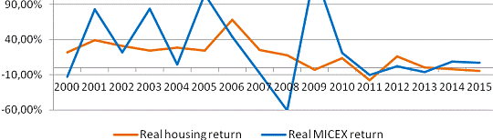 . 1. Real return of residential
housing vs. real return of financial market 1998-2015
. 1. Real return of residential
housing vs. real return of financial market 1998-2015
real estate
market is highly opaque because of incredible amount of factors that influence
the price, which are studied in hedonic models such as (Goodman 1978),
(Malpezzi and others, 2003), etc. This aspect complicates research in
this field, especially macroeconomic and regulatory aspects are currently
underinvestigated. In particular, little had been done for understanding real
estate market in Russia despite the fact that questions connected to pricing of
such assets are urgent for Russian investors as well as for any other investors
in the world. past years housing prices in Russia were quite volatile (see
figure 2). Before the recent global economic crisis they rocketed due to not
only general upward trend in the Russian economy with all its consequences in
the form of rising personal income, easing of credit conditions, etc. but also
due to mortgage loan market expansion. Mortgage
mass market appeared in Russia in 2005 and the financial product became popular
very soon: in 2006 there was a considerable real estate demand increase which
pushed pricesup in average by 48%. However during the crisis of 2008-2009
prices had plummeted down up to 42% (in Kirov region) and since then they are
recovering but with much slower paces compared to pre-crisis period.
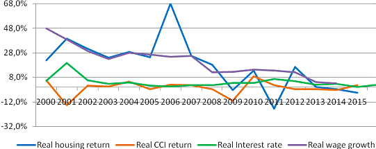
Fig.2. Real
return of RE compared to real growth of construction costs, wages and interest
rates
the
importance of these fluctuations’ consequences for the Russian economy this
topic was not really popular among researchers. As one could have noticed
before crisis of 2008-2009 real housing prices appreciated much faster than for
example such supply-side factor as growth of production costs or traditional
demand-side price driver - real disposable income (named wage on the graph).
And after the crisis culmination prices plummeted also faster than all those
indicators. The questions about was the housing market in equilibrium at that
time and what was the mechanism of price adjustment to the shocks that occurred
during that period are still unanswered. Howeverthey become increasingly
important because of current economic instability in Russia which provokes the
similar type of shocks that have already happened several years ago. That is
why the further research of housing pricing mechanism in Russia is an urgent
issue. majority of research papers are devoted to real estate indexes design,
real estate value estimation and real estate portfolio management. Some studies
are aimed at finding prices or return determinants, e.g. papers written by Ball
(1973), (Hirata et al. 2012), (Krainer and Wilcox 2013). Whatsoever there is no
convincing theory behind them, which means that value drivers that had been
found significant are appropriate for each particular region in certain time
period and cannot be considered as fundamental factors. This leads to the
conclusion that simple rearrangement of variables in the equations is not the
most efficient tool not only for understanding the market but especially for
forecasting purposes. Therefore in order to investigate housing price dynamics
more comprehensive approach that would consider equilibrium formed under demand
and supply influence is needed. That is why the purpose of this study is stated
as follows: to develop anequilibrium model of residential real estate markets
in Russian regions. To achieve this goal several steps should be implemented.
Firstly, a
review of the recent studies that describe operation mechanism of real estate
market including participants, their goal and behavior on that market;
exogenous factors that can influence equilibrium on local housing market;
channels through which the regulation of the market is implemented. Secondly,
based on the result of previous research the relevant assumptions about
economic agents that participate inprice formation process on the housing
market in Russia should be made and theoretical model of the housing prices
should be developed. After that hypotheses of the research need to be
formulated and the relevant data should be collected in order to test whether
theoretical model developed beforehand fits the empirical data and to test
stated hypotheses. After the model parameters assessment, the conclusions about
model preciseness will be made and limitations will be discussed.
The results
of the study are expected to be useful for the whole understanding of housing
pricing mechanism in Russia including how different economic agents participate
in price formation making their day-to-day decisions, how housing prices would
change if some sort of market shock occurred or how the regulator can influence
prices through different channels. Therefore the results of the study
can be implemented by almost all types of economic agents: from citizens
concerned with the question is it worth buying additional real estate unit to
Russian regulatory forces such as the Central Bank of Russian Federation or the
Ministry of Finance and investors who have long-term investment horizon, such
as pension funds, developers or other investors.
Basic issues about housing prices
formation process
Historically real estate in Russia performed as
an alternative way of savings instead of financial assets such as stocks,
bonds, deposits, etc.Prices of residential housing for extended periods rose at
least with inflation paces or in some periods even much faster, and during
crises real estate value dropped significantly less than the value of most
financial assets.Therefore real estate can be considered as non-traditional
store of value however it is not that any real estate object can be deemed as
an investment asset. order to define what we are going to consider as an asset
on real estate market let’s turn to legislation. According to the Civil Code of
Russian Federation (article 130, Civil Code of RF) «The immoveable property
includes plots of land, subsoil and all that is firmly connected to the ground,
that is objects that cannot be moved without disproportionate damage to their
usability, such as buildings and construction objects in progress, aircrafts
and sea vessels, inland navigation and space objects». Within the framework of
this research only those pieces of real estate that can be inhabited will be
studied, that is why among all of the real estate objects only buildings will
be taken into account. estate is divided into two groups: commercial and
residential property. Some high-class business center is an example of
commercial real estate; its main distinguishing feature is generation of a rent
for owner. Houses and apartments in order to live are the residential property.
Even if a private owner of real estate decides to rent it, the house, flat or
land plot does not become commercial property. Due to the fact that commercial
property generates cash flows its pricing is dependent from dynamics of these
flows that in turn are majorly influenced by the variety of factors individual
for each piece of property such as, for example, purpose of using (e.g.
warehouse, office center, etc.). So it could be concluded
that commercial property even more heterogeneous than residential property,
pricing of different types of objects differs and therefore it is hard to
determine fundamental factors. Therefore, within the framework of this research
only pricing of residential houses will be studied.
Besides real estate market like equity market
can be divided into primary and secondary segments. Primary real estate market
implies selling the object to its first owners. Usually these objects are
buildings in progress or new buildings, which can be bought straightly from the
developer. In opposite, real estate objects that already had at least one owner
are traded on the secondary market. Despite the fact that both - primary and
secondary real estate markets - are highly heterogeneous within themselves,
primary market can be considered as even more heterogeneous than secondary.
Developers can offer apartments without finishing, with primary finish or with
full decoration depending on needs and wishes of buyers. Each type has its own
average price that is why within this research secondary real estate prices
will be studied.in real estate market is highly opaque.There are several
reasons for that. Information asymmetry is higher on this market in comparison
with other traditional financial assets (stocks, bonds, currency, etc.)
markets. The reason why this happens is that for external investor it is time
consuming and costly to carry out a comprehensive assessment of real estate
objects, poor information can be obtained from open sources. Moreover there is
nosuch financial institute in Russia as Real Estate Investment Trusts that
operate in the USA, which means that real estate is not traded on exchange,
there is only low-liquid private market.
These issues
motivated the classical and widely known research conducted by Karl Case and
Robert Shiller «The efficiency of the market for Single-Family Homes», where
week-form efficiency of the residential housing market was tested. Authors
found an empirical evidence of prices inertia on American real estate market,
which means that prices theoretically can be predicted based on the previous
history. (Case and Shiller 1988)This result found implications in
furtherdynamic models of housing market of different countries such as
(Poterba, Weil and Shiller, 1991) and in particular in dynamic models of
general equilibrium such as (M. Iacoviello 2010)(M. Iacoviello and Neri 2008),
etc.conservative way of housing prices drivers’ determination is reduced-form
models estimation which usually implies analysis of panel (Tsatsaronis and Zhu
2004) or time series data (Rosen and Topel 1986) in order to find statistical
correlation between housing prices and other different variables or to find
predictability of prices in the past. to the fact that residential housing is
highly heterogeneous not only between the regions but also within them, there
are few markets studied on wide, at least cross-regional, sample. Also it
should be noted that the irregularity of the following sort exists: simple
reduced-form models were proposed for both developed and developing regions and
no coherent result was obtained. There are almost no similar factors that drive
the prices in these two types of markets and furthermore one could have noticed
that correlations between so-called fundamental factors such as GDP growth,
unemployment rate, ageing, etc. are unstable in the time (see appendix
1).instance the research conducted by (Krainer, Wilcox 2013) proved that the
Hawaii regional housing market was boosted by the Japanese who massively moved
there and made heavy contribution in the GRP of the region. Other research of
American regions such as(Calomiris, Longhofer, and Miles 2013)or (Hwang and
Quigley 2006) showed the opposite - in average GRP growth appeared to be
irrelevant for housing market, presumably due to the fact that mortgage
conditions were more powerful driver at the period under study. the question
“is GDP a fundamental factor of housing prices?” is not the only controversial
issue. The causal relationship of GDP and housing price also can be questioned:
for example right before the recent crisis of 2008-2009 Edward Leamer wrote his
famous paper alleging that residential housing market defines medium term
business cycles and supported that hypotheses with persuasive empirical
results. (Leamer 2007) However this paper caused a wave of counter-research
such as for example the paper of (Ghent and Owyang 2010) that stated the
opposite causation. And this is the only one of many cases of inconsistencies
that exist in the research field, which one more time emphasize the importance
of reliance on economic theory first and on the empirical evidence further.form
analysis is more widespread compared to structural modeling and the majority of
early or even current research papers are based on results obtained with help
of this method.However this type of models usually relies on unrealistic
assumptions about data features and economic agents behavior, furthermore it is
widely known that correlations does not imply causation. It could be noted that
determinants of housing prices which have already been found by researchers
vary from country to country and from period to period.number and the structure
of indicators that were proved to be price or return predictors are also different
in listed studies, which mean that there is still no unanimity between
economists on what factors should be considered as fundamentals, because there
is thin theoretical background behind these reduced-form models. Moreover these
models can capture the influence of observable variables, some unobserved
parameters can only be substituted with help of proxy indicators that can be
inaccurate or cannot be traced at all (for instance, such behavioral parameter
as risk-aversion). drawbacks can be mostly eliminated with help of structural
modeling which puts the economic model first and econometrics after, so this
type of models allows relying on causation a priory. Besides they allow
assessment of unobserved parameters comparing theoretical, economic model with
observed empirical data. Moreover with help of such tools of estimation the
researcher can answer different types of questions such as “what happens in the
case of some shocks?” or “what happens if there is s systematic shift, for
example if regulator decided to increase key rate or profit tax rate?”. Ability
to estimate that type of influence makes results of the model estimation more
interesting, viable and useful for practical, including regulatory, purposes.
In order to investigate what had been done in this research field let’s study
the literature devoted toestimation of housing market structural models. The
most relevant papers are presented in the table 1 below.pioneer of structural
equilibrium studies on housing market was the paper of James Poterba published
in 1984 where the dynamic interconnection of inflation expectations, housing
prices and housing stock was described within the intertemporal model of
individual wealth accumulation. This research allowed drawing several
conclusions. First of all, it showed that households solving the optimization
problem given the inflation expectations make more significant contribution in
housing price formation than suppliers. Secondly, residential real estate
prices are the core drivers of construction investment activity. Finally, the
model allowed the simulations of tax-subsidies effect on the market. the
importance of this study for the formation of new trend in real estate research
it was heavily criticized for a number of reasons. In particular the author
ignored cost structure of construction - this problem was fulfilled in other
papers such as for example (DiPasquale and Weaton, 1997), where the land cost
was outlined as a matter of special importance. Despite the fact that
theoretical framework described in that paper as a whole was proved to be
consistent, cost structure empirically was insignificant for price formation
process, probably because of non-suitable proxy for land costs (the researchers
used price of farm land). This problem was solved on the New Zealand data in
the study of(Grimes and Aitken 2010), who used an actual residential
construction land cost. For other markets the issue is still underinvestigated
due to unavailability of proper data. the irrelevance of supply which was
stated by Poterba had been challenged by a number of studies such as(Caldera
and Johansson 2013)and (Glaeser, Gyourko, and Saiz 2008). Construction
constrains were proved to explain instantaneous stickiness of the housing
prices in dynamic models. Due to the fact that the amount of vacant land which
is suitable for residential construction is highly restricted especially in
metropolitan areas, it takes time and considerable amount of resources to pass
through all the governmental procedures to obtain a building permit and start
construction works.
Table 1. Literature review on
empirical estimation of housing market structural models
|
Article
attributes
|
Sample
|
Variables
and Method
|
Results
|
Housing
market spillovers : evidence from an estimated DSGE model (M. M. Iacoviello
and Neri 2008)USA
1695-2006 quarterly dataDSGE model. The goal: to study core
drivers of housing prices in the USA; to study the effect of housing market on
external economic environment: prices are mostly driven by the availability of
land and the difference in technological progress between housing and
non-housing sectors; monetary factors explain only 20% of housing price
variation;
|
Wage rigidity increases the sensitivity of
output to shifts in aggregate demand; collateral effect increases the
elasticity of consumption to wealth. So spillovers of the housing market
matter more and more
|
|
|
|
|
Supply constraints and housing market dynamics
(A.
Paciorek, 2013)
|
USA
1975-2008 yearly data
|
Dynamic
structural model
|
The goal: to investigate the mechanism of
interconnection between housing supply and housing prices Results:
bureaucratic processes diminish developer’ reaction on demand shocks and
create additional expenses for them; geographic limitations restrict
opportunity for quick response for demand shocks which leads to housing
prices volatility
|
Housing
Bubbles and Busts: The Role of Supply Elasticity (Ihlanfeldt and Mayock
2014)63
counties of Florida, 1990-2010 yearly dataHousing supply Stock-adjustment model
The goal: to find a solid way of supply elasticity calculation; to find key
determinants of housing supply elasticity in Florida counties
|
Results: the most solid approach is
repeated-sales method; elasticity depends on the amount of undeveloped land,
planning expenditures and average housing value. Key determinants vary
depending on the period under observation - boom or burst on the housing
market.
|
|
|
|
The model of
housing in the presence of adjustment costs: a structural interpretation of
habit persistence (M.Flavin;
S. Nakagawa 2001)USA 1975-1975 yearly dataStructural modeling, GMM estimatedThe
goal: to investigate whether consumers’ habit persistency and the presence of
adjustment cost play a significant role in housing price formation process
|
Results: little evidence of habit persistence
influencing consumers’ choice were found; estimated substitutability between
housing and perishable goods is very low
|
|
|
|
Consumption,
house prices and collateral constraints: a structural econometric analysis (M.
Iacoviello 2005)USA 1986-2002 quarterly dataStructural modeling, GMM estimatedThe
goal: to study the effect created by housing prices shocks on consumption
throughout borrowing capacity tightly related to real estate value
|
Results: home equity gains can be transferred
into higher borrowing and higher consumption (the parameter of elasticity was
estimated)
|
|
|
|
A dynamic
model of housing demand: estimation and policy implications (Bajari et al.
2013)USA 1975-2009 yearly dataReduced-form estimation: Multinomial
Logit and panel regression; Structural modeling: non-parametric estimationThe
goal: to specify, estimate and simulate structural model of housing demand
(considering the effect of the following variables: adjustment costs, credit
constraints, uncertainty about evolution of income and housing prices)
|
Results: during price or income shocks
households reduce the consumption of non-durable goods and their wealth as
well in attempt to keep their houses and avoid adjustment costs associated
with buying or selling of real estate
|
|
|
|
|
Modeling structural change in the UK housing
market: a comparison of alternative house price models (N.Pain,
P.Westaway, 1997)
|
UK
1968-1990 quarterly data
|
VAR modeling, Dynamic structural modeling,
|
The goal:to develop a new approach to the
modeling of housing prices in the UK, considering consumer expenditures as a
main determinant of real estate demand Results:created model appeared to be
more consistent in comparison with conservative models such as NIDEM or HM
Treasury Model
|
The dynamic
relationship between housing prices and the macroeconomy: evidence from OECD countries
(Kishor and Marfatia 2016)15 OECD countries 1975-2013 quarterly dataError-correction
model, Dynamic OLS estimatedThe goal:to find fundamental macroeconomic
determinants of housing prices by decomposition of prices movements into
permanent and transitory components
|
Results:income and interest rate are the
forces that provoke long-run changes in the housing prices in OECD , other
factors influence was classified as transitory
|
|
|
|
Tax
subsidies to owner-occupied housing: an asset-market approach (Poterba
1984)USA 1974-1982 quarterly dataReduced-form nonlinear rational
expectations modelThe goal:to study inflation’s effect on the tax subsidy to
the owner occupation as a factor of housing prices volatility
|
Results:tax subsidies alongside with rising
inflation rate reduce the real mortgage expenses and boost housing prices;
the core driver of supply was the real price of houses
|
|
|
|
Market
thickness and the impact of unemployment on housing market outcomes (Gan and
Zhang 2013)Texas (28-38 cities), 1990, 2000 and 2010Structural
model, non-parametric estimationThe goal:to identify the channel through which
unemployment affects the housing market considering the thickness of this
market
|
Results:unemployment generates thinner
marketwhich leads to the poorer matching quality, and as a consequence
housing prices decrease more than if there were no thickness effect
|
|
|
|
|
House prices since the 1940s: cointegration,
demography and asymmetries (S.Holly, N.Jones, 1997)
|
UK,
1939-1994
|
Error-correction model, OLS-estimated
|
The goal:to develop a broader vision of UK
housing market, to observe it for the long period of time during different
business-cycles and different inflation conditions and to develop a long-run
model for it Results:the core determinant of housing prices in the long-run
is real income, the influence of other factors such as the change in
demographic pattern or the rise of building societies was more serious when
housing prices deviated too much from equilibrium level implied by real
income
|
Housing
Supply, Land Costs and Price Adjustment (Grimes and Aitken 2010)New
Zealand (regional-level data), 1991-2004 quarterly data Error-correction model,
MLE estimatorsThe goal: to explore the mechanism connecting housing supply
elasticity, land costs and housing prices response to various shocks, e.g.
demand shock or bubble
|
Results: The higher relative cost of
construction land unit, the more inelastic supply is and therefore the more
volatile housing prices (demand shocks deviate prices for a long time from
their equilibrium values)
|
|
|
|
idea of residential land rarity
inspired a new branch within the residential real estate research field -
spatial equilibrium models that currently focused on the equilibrium urban
growth model developed by(Capozza and Halsley, 1989). As a result the
importance of the interaction of the supply and demand in the housing price
determination was proved in previous research so both of the market sides
should be studied on the Russian market as well. core problem in structural
equation modeling is to construct an appropriate functional form of the
equations. This means not only the compliance of the model to common sense and
economic theory, but also that the model needs to be “estimateable”. For
instance, ordinary data procession technics such as General Method of Moments
(GMM) or Maximum Likelihood estimation can be applied only to the closed-form
equations sets where the number of endogenous variables corresponds to the number
of equations so the system can be solved with the only one set of parameters’
values. Anyway even if the model could be properly estimated it still can
appear inconsistent when tested on the empirical data.
Each author
or the set of authors suggested different variations of the model that would
describe the housing market. After the publication of Poterba’s results many
research papers were mainly devoted to demand function estimation. Most of them
modeled the behavior of the representative household that at each point of time
decides whether to stay in the current accommodation or move to the bigger one,
continuously maximizing its’ expected lifetime utility on the condition of
constrained personal income. The majority of housing equilibrium research such
as (Beaulieu, 1993) which was one of the first who connected durable and
non-durable consumption under one utility function and after that(M. Iacoviello
2004), (Grimes and Aitken 2010) and others started using the utility function
based on consumption CAPM model developed by(Mankiw and Shapiro, 1984). And
this approach was proved to be empirically relevant for many regional US
markets. an extension of housing demand model(M. M. Iacoviello and Neri 2008)
suggested differentiate households by their ability to safe into patient (those
whosave money until they decide to expand their living space, and therefore
those who lend their savings through financial assets) and impatient (those who
increase current consumption and therefore are forced to borrow money when they
decide to buy a new square meters of real estate). These types have different
constraint functions but the same anticipations about the future states of the
world, so the model is more complex than traditional one but still solvable.
set of authors (Flavin and Nakagawa 2001) supplemented to the theory of (M. M.
Iacoviello and Neri 2008)with the presence of adjustment costs and habit
persistence when household makes a decision to move.The model proposed by the
authors suggests that these costs decrease the elasticity of demand for housing
which makes the process of price adjustment more difficult and prices
themselves more volatile. Despite the fact that the model was constructed with
accordance to the strict economic logic the empirical evidence of the
importance of adjustment costs was not found which supports the statement that
even theoretically solid model can be wrong.things considered, most attempts to
significantly complicate the initial equilibrium model on the national or
regional housing market were not persuasive enough for considering such
theoretical functional forms of supply and demand equations as valid. Some of
them just failed empirical testing, others were proved to be significant but
only for a certain territories (for instance some states of the USA or New
Zealand) and certain periods of time. That is why within the framework of this
research classical set of assumption about economic agents’ behavior would be
implemented. Which means that all the households as well as construction firms
would be considered as identical, therefore they would have the same
anticipations about future and the same utility function and total costs
function. is also worth noticing that research conducted under structural
equilibrium approach is a standard for developed countries mainly for USA
housing market (see table 1). Despite all the advantages of structural
estimation modeling before reduced-form models there are few (if there is some)
papers devoted to studying housing market of developing countries. Especially
rare this type of research is for Russian market because of the number of
factors such as for example unavailability of durable data, because the
earliest data which could be obtained from official sources starts from 1996.
That means that the researcher now can observe all-transactions housing price
index only for 19 years, whereas the analogous indicator for USA market is
available since 1975, i.e. 40 years. Besides, mortgage market statistics in
Russia is available only since 2005, whereas the majority of indicators
describing the situation on mortgage market of the United States cover the
whole observation period of housing prices. , there is such a data source as
United States Census Bureau which allows getting comprehensive information on
representative households’ behavior for vast period of time, so the
ready-to-use panel dataset is available for the researchers. This dataset
allows analysis of housing market on the base of repeated sales basis, Russian
statistical services bureau do not use such a methodology - only average level
of deal prices is calculated.is no centrally accumulated dataset of indicators
describing Russian consumers’ behavior, all the information need to be
collected by hands from different sources of information such as official sites
of Russian Federal and Regional Statistics Services, Central Bank of Russian
Federation and sites of different Ministries. Therefore, only fragmentary
representation of such behavior in particular regarding housing market can be
observed. Anyway all those difficulties could be overcome by applying
sufficient effort and resources.sum up, Russian housing pricing mechanism is
underinvestigated, fundamental factors that influence prices were not defined
in the previous research papers. That is why this study will be devoted to
formalization of housing price formation process through the finding the
appropriate functional form of regional housing supply and demand. This means
not only finding indicators that make their contribution in consumers’ demand
or in construction activity, but also finding the channels through which they
participate in the residential real estate pricing process. the research
question of the study can be formulated in the following way: what are the
fundamental driving forces of housing prices in Russia? Achievement of the
research goal and finding the answer to the stated question will make it
possible not only to conclude about factors that influence prices but also to
judge whether prices where in equilibrium during the whole period in study.
Equilibrium models can also be useful for making projections about prospective
of the housing prices in Russian regions and for regulation purposes as well.
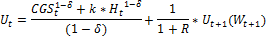
model of
housing prices
function’s
assume that there are N (= workforce*employment level) identical individuals
(all those who earn income and can spend it on consumption and saving) with
homogenous utility function and expectation about future states of the world.
Each of them earns a certain amount of money in any form - salary, rent or
profit. The representative individual in each period divides the income between
current consumption of goods and services including for example such durable
goods as household appliances, cars, etc. and savings in the form of either
housing consumption or financial assets. So the budget constraint of the
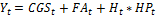
representative household can be written as following:
|
|
(1)
|
Yit is a total income at t-th period
(average monthly value for each year); CGSt is a value of fixed set of goods
and services at the t-th; FAit is an amount of individual’s spending at the
t-th period of time on financial assets such as stocks, bonds, deposits, etc.;
Ht is a quantity of housing consumed at the time t; HPt is a housing prices at
the time t.to the fact that accumulation of capital assets is associated with
some of rate of return and at the same time real assets such as house or flat
depreciate with time, the intertemporal constraint for individual wealth can be
formulated as follows:
|

|
(2)
|
Wt is accumulated by t-th period
amount of individual wealth;  is a real
after-tax rate of return on financial assets (FAt);
is a real
after-tax rate of return on financial assets (FAt);  is
a cost of borrowing money for buying real estate - mortgage rate; d is a rate
of housing depreciation (for simplicity let’s assume that it constant across
all the periods);
is
a cost of borrowing money for buying real estate - mortgage rate; d is a rate
of housing depreciation (for simplicity let’s assume that it constant across
all the periods); 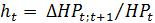 - growth rate of
real housing prices between (t+1)-th and t-th periods.
is assumed to be exogenous in this model framework, because the existence of
competitive financial market is suggested. individual gets utility from current
consumption of durable and non-durable goods as well as from consumption of
housing services. Under housing services the convenience of possession instead of
renting real estate will be meant, so this variable is unobservable. Therefore
it was assumed that the value of housing services is proportionate to housing
stock per person with some coefficient - k. The utility function which is
identical for all the individuals is derived from Consumption CAPM model and it
is convex function with constant relative risk-aversion, which can be presented
in the following way:
- growth rate of
real housing prices between (t+1)-th and t-th periods.
is assumed to be exogenous in this model framework, because the existence of
competitive financial market is suggested. individual gets utility from current
consumption of durable and non-durable goods as well as from consumption of
housing services. Under housing services the convenience of possession instead of
renting real estate will be meant, so this variable is unobservable. Therefore
it was assumed that the value of housing services is proportionate to housing
stock per person with some coefficient - k. The utility function which is
identical for all the individuals is derived from Consumption CAPM model and it
is convex function with constant relative risk-aversion, which can be presented
in the following way:
|
|
(3)
|
rational individual maximizes his
utility with respect to current consumption and housing consumption - the
variables that he can choose and vary every period. Solving the maximization
problem taking into account intertemporal wealth constraint one could obtain
the following equality, which reflects the optimal ratio of housing consumption
with respect to current consumption:
|
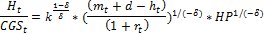
|
(4)
|
Calculus appendix.
|
|
(5)
|
|

|
(6)
|
|
 (7) (7)
|
|
By dividing first-order conditions
to each other and by expressing the variable of interest  with
help of other variables, individual demand function will be obtained.order to
make this demand function aggregate, let’s sum it up over N consumers and solve
it with respect to h, which means finding inverse demand function
with
help of other variables, individual demand function will be obtained.order to
make this demand function aggregate, let’s sum it up over N consumers and solve
it with respect to h, which means finding inverse demand function
(8)
(9)
|
linearization, let’s rewrite the
equation in the logarithmic form considering the fact that all values under
logarithm are not negative in accordance with their economic sense
|

|
(10)
|
should be noted that within the
model all the consumers as well as developers for simplicity will be
price-takers - none of them as a single agent cannot significantly influence
the average price of real estate formed on the market. For future research in
this field it can be suggested observing other industrial structures other than
perfect competition, because construction and development is an industry with
high barriers. That is why regional market most likely takes form of oligopoly
with a few big players that can interact with each other in many different ways.for
real estate in each particular region is presented majorly by the population of
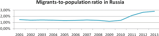
this region. Due to the fact that interregional mobility in Russia is not high
(see picture 1 below) - from 1.33% to 2.8% of total population during the
period from 2001 to 2013, and 1.63% in average - within the framework of this
study interregional demand for real estate will not be considered. Therefore
demand in the region is created by inhabitants of the region and cross-regional
demand component is omitted out of the model.
due to the fact that competitive
construction and development market was assumed, it can also be suggested that
cross-regional housing supply is negligible. Competitive market structure
implies zero economic profit and low industry entrance barriers, so if there is
an excessive profit in some region firms from other regions instantaneously can
use this situation for additional financial gains until there is no such gain.
Therefore profitseventually become equal among regions again and that is why
cross-regional supply can be omitted out of the model as well.
Supply function
homogenous construction and
developing firms form the regional housing supply. Each of them decides to
built additional housing up to the point where their replacement costs that can
be determined as full cost of construction of a new house per one square meter
are equal to the expected market price at the period of sale - let it be period
t+1. Let’s assume that all the construction costs can be divided into capital
expenditures including cost of materials, machinery, construction and
installation activities; labor expenditures which can be approximated by
average salary and cost of borrowing betweenperiods t and t+1.can be suggested
that labor and capital can be considered as substitutes to some extent in the
process of real estate building - for example, the company can rent special
equipment such as elevators, concrete mixers, etc. to meet their construction
deadlines or it can just employ more workers, however both types of these
expenditures should be incurred in order to build a house. Therefore the total
cost function can be constructed as some sort of Cobb-Douglas function with
constant return to scale:
|

|
(11)
|
 is a
region-specific proportion coefficient which reflects the extent of total cost
inflation if capital and labor prices go up;
is a
region-specific proportion coefficient which reflects the extent of total cost
inflation if capital and labor prices go up;  is
average capital expenditures in i-th region at t-th period;
is
average capital expenditures in i-th region at t-th period;  is
average labor expenditures in i-th region at t-th period; α
and (1-α)
are total cost elasticities of capital costs and labor costs respectively; is
a financial cost for t-th period which is equal among all the regions because
there exist the unified national financial capital market. companies in each
region (denoted by index i) form their expectation about the future period t+1
based on the all information available to them at the period t -
is
average labor expenditures in i-th region at t-th period; α
and (1-α)
are total cost elasticities of capital costs and labor costs respectively; is
a financial cost for t-th period which is equal among all the regions because
there exist the unified national financial capital market. companies in each
region (denoted by index i) form their expectation about the future period t+1
based on the all information available to them at the period t -  where
where
 is
an information set of t-th period. Current housing prices and cost of funding
will be considered as exogenous for companies, because of competitive market
structure. Expectations of construction firms are based on the current market
situation, but also they can consider region-specific factors such as general
growth of GRP, mortgage subsidy program, etc. and time-specific effect related
to nation-wide economic cycles. So expected prices will be defined in the
following way:
is
an information set of t-th period. Current housing prices and cost of funding
will be considered as exogenous for companies, because of competitive market
structure. Expectations of construction firms are based on the current market
situation, but also they can consider region-specific factors such as general
growth of GRP, mortgage subsidy program, etc. and time-specific effect related
to nation-wide economic cycles. So expected prices will be defined in the
following way:
|

|
(12)
|
 is a
regional-specific growth factor calculated as a function of Gross Regional
Product (GRP) growth rate;
is a
regional-specific growth factor calculated as a function of Gross Regional
Product (GRP) growth rate;  is time-specific
growth factor;
is time-specific
growth factor;  and
and  are
associated coefficients. GRP is considered as an exogenous variable within this
model - despite the fact that construction and development companies
participate in GRP formation, their influence is negligible within the whole
regional economy. to the fact that secondary real estate market is observed in
this study, the main indicator of supply is real estate stock which is
available at a certain moment in time, which can be calculated as follows:
are
associated coefficients. GRP is considered as an exogenous variable within this
model - despite the fact that construction and development companies
participate in GRP formation, their influence is negligible within the whole
regional economy. to the fact that secondary real estate market is observed in
this study, the main indicator of supply is real estate stock which is
available at a certain moment in time, which can be calculated as follows:
|
|
(13)
|
- real estate stock, available by
the end of period t; SoDt - size of dwelling for period t;UHt - value of
uninhabitable real estate for period t. change of housing supply in t-th period
can be defined as a difference between size of dwelling and the disposal of
uninhabitable housing in the i-th region at t-th period. Therefore the growth
rate of housing supply at t can be calculated as:
|
 , ,
|
(14)
|
Where  is
a rate of housing supply growth between period t and t+1 in i-th region;
is
a rate of housing supply growth between period t and t+1 in i-th region;  is
a size of dwelling that had been started at t-th period and was offered for
sale at t+1 at i-th region;
is
a size of dwelling that had been started at t-th period and was offered for
sale at t+1 at i-th region;  is a size of
uninhabitable residential real estate which was removed from housing market;
is a size of
uninhabitable residential real estate which was removed from housing market;  is
a housing stock available at the market at t-1 period.supply can be determined
as a function of expected real estate prices relative to full replacement cost
of construction according to Q-theory formulated by J. Tobin. In the context of
real estate market this theory implies that construction firms make their
investment decision to build a house based on benefit-cost analysis: they build
additional housing is expected prices are higher than current total costs. Therefore
housing supply equation will be determined as follows:
is
a housing stock available at the market at t-1 period.supply can be determined
as a function of expected real estate prices relative to full replacement cost
of construction according to Q-theory formulated by J. Tobin. In the context of
real estate market this theory implies that construction firms make their
investment decision to build a house based on benefit-cost analysis: they build
additional housing is expected prices are higher than current total costs. Therefore
housing supply equation will be determined as follows:
|
|
(15)
|
taking a logarithm of both
right-hand and left-hand sides for linearization and by substitution of  and
and
 with
correspondinglogarithmic expressions, the following log-linear supply function:
with
correspondinglogarithmic expressions, the following log-linear supply function:
|
 , ,
|
(16)
|
 is price elasticity
of supply parameter;
is price elasticity
of supply parameter;  is a coefficient
which reflects the influence of region-specific factor;
is a coefficient
which reflects the influence of region-specific factor;  is
a coefficient which reflects the influence of time-specific factor;
is
a coefficient which reflects the influence of time-specific factor;  is
an overall error term.appendix:’s create a logarithmic form of expected housing
prices and total costs equations:
is
an overall error term.appendix:’s create a logarithmic form of expected housing
prices and total costs equations:
|

|
(17)
|
|

|
(18)
|
form of housing supply equation is:  .
By substitution of two former expressions into supply function, the following
log-linear form of housing supply will be obtained:
.
By substitution of two former expressions into supply function, the following
log-linear form of housing supply will be obtained:
|

|
(19)
|
final form of housing supply
equation can be obtained by grouping items on the basis of their compliance -
mathematical and economic.
formulation
theoretical framework that was
formulated above is based on the plain idea of equilibrium between supply and demand(see
figure 3), which are formed in turn under the influence of outlined
characteristics of the whole Russian economy, regional specific features and
personal characteristics of individual households.
Fig. 3. Graphic representation of
the theoretical modelinfluence of the national economy as a whole is
represented by borrowing and lending terms: loan rate for construction and
developing companies which is suggested equal to the rate of return at which
households invest their funds and mortgage rate for households. Despite the
fact that mortgage rate varies over the regions it is based on the Russian key
rate which defines the cost of the money in the economy and on observed and
expected inflation rate. That is why mortgage rate can be considered more as a
factor reflecting the situation in the whole economy rather than in the
separate regions. coefficient  included into the
demand function reflects the relative expensiveness of investing in the housing
(which presented by cost of borrowing (mt) and depreciation rate that assumed
to be constant over time and regions) instead of placing saved funds in
financial instruments that brings some rate of return - rt. So the higher costs
of buying of an additional real estate the lower demand should be which
eventually would depress housing prices. : The higher relative costs of buying
real estatecompared to an alternative rate of return the lower housing prices
arethe influence of business cycle and the overall trend in the economy is
accounted in the supply function through time-specific effect. The presence of
this effect implies a positive trend in housing construction, which could
include technology improvement over time which allows building real estate
faster and/or cheaper, the increase of labor productivity or the fact that over
time population becomes richer due to for instance trade unions activities and
increase of minimal wages. All these factors can facilitate the increase of constructors’
profit margins and push prices higher relative to the cost of construction
dynamics. So the positive influence of time factor which is included into the
expected price formation process goes without saying. regional-specific factors
of demand there are working force of the region, employment level and housing
stock of the region. Due to the fact that housing stock is naturally higher for
regions with higher population, it was scaled by employed population of the
region (those who create efficient demand). So real estate stock per capita is
included in the demand function. The law of demand connects the price of real
estate and the amount of the occupied housing: the higher the price is, the
lower the amount of housing is purchased. regional-specific growth factor
calculated as (1+ GRP growth rate) in the supply function as a part of
anticipations of construction companies about future prices. The dynamic of
production which accurately reflects the situation in the economy appeared to
be highly significant in the majority research papers such as (Grimes and
Aitken, 2004), (Kishor and Marfatia, 2016), (Berger et al, 2015) and some
others. So the assumption about fact that economic agents base their
expectations on the past was validated. However these models were tested on
quarterly data so it could be concluded that this result was proved only for
short-term periods. Besides the significance was shown mainly for developed
countries and on country-wide data, the importance of cross-regional
differences has not been yet tested for developing countries. Therefore the
following hypothesis can be suggested. : Gross Regional Product plays
significant role in the formation of price expectations on housing market in
Russian regionstotal cost function of construction companies is based on the
distribution of expenses between human and capital resources. So theoretically
this function should be individual for each company. Howeverdue to the
existence of the assumption about competitive industrial structure all the companies
are price-takers on the labor market and market of construction materials,
machinery, financial resources, etc. And considering regional economy level
this assumption seems to be reasonable because if there was higher than average
salary in the construction industry there would be an inflow of workers on that
market and wages would converge to the average level. Therefore the average
regional value of such variable as labor cost and capital cost were used.
Anyway themore expensive resources to the company relative to the anticipated
housing prices are the less incentive to build additional living spaces
constructors and developers have.: The inflation of total cost which is not
supported with corresponding increase of housing prices holds back construction
activityof unavailability of information about cost structure of each builder
in each region such cost equation coefficients as the elasticity of
substitution (alpha) and proportion coefficient (gamma) are unobservable and
therefore impossible for separate estimation. They are assumed as constant and
would be incorporated into estimated empirical parameters of the linear supply
function.individual features that participate in the demand formation there is
a share of current consumption of perishable and non-housing durable goods in
the households disposable income (not only wage, but rent, profit from
entrepreneurship or any other type of income). Housing consumption and
consumption of goods and services are connected through the income constraint which
means that the household have to distribute its income between these positions
-if it spends more on current consumption it has less to invest in housing. At
the same time the law of demand implies inverse relationship between the amount
of housing purchased and the price of housing. Therefore the lower demand for
real estate is the higher the prices are. That is why theoretical model
formulated beforehand suggests that housing prices and consumption of goods and
services are connected directly to each other. the fact that all the
unobservable variables in the demand equation such as the risk-aversion and
coefficient of housing services are theoretically individual to each household
there is no ability to measure them separately for every individual and
therefore test hypotheses about their influence. That is why these coefficients
considered as constant in the equation and therefore will be incorporated into
the estimated parameters of the empirical model.order to test whether developed
theoretical model describes the real situation on the regional housing market
in Russia the appropriate data should be collected from reliable sources of
information. The process of data collection and discussion of data features are
presented in the following sections.
included into the
demand function reflects the relative expensiveness of investing in the housing
(which presented by cost of borrowing (mt) and depreciation rate that assumed
to be constant over time and regions) instead of placing saved funds in
financial instruments that brings some rate of return - rt. So the higher costs
of buying of an additional real estate the lower demand should be which
eventually would depress housing prices. : The higher relative costs of buying
real estatecompared to an alternative rate of return the lower housing prices
arethe influence of business cycle and the overall trend in the economy is
accounted in the supply function through time-specific effect. The presence of
this effect implies a positive trend in housing construction, which could
include technology improvement over time which allows building real estate
faster and/or cheaper, the increase of labor productivity or the fact that over
time population becomes richer due to for instance trade unions activities and
increase of minimal wages. All these factors can facilitate the increase of constructors’
profit margins and push prices higher relative to the cost of construction
dynamics. So the positive influence of time factor which is included into the
expected price formation process goes without saying. regional-specific factors
of demand there are working force of the region, employment level and housing
stock of the region. Due to the fact that housing stock is naturally higher for
regions with higher population, it was scaled by employed population of the
region (those who create efficient demand). So real estate stock per capita is
included in the demand function. The law of demand connects the price of real
estate and the amount of the occupied housing: the higher the price is, the
lower the amount of housing is purchased. regional-specific growth factor
calculated as (1+ GRP growth rate) in the supply function as a part of
anticipations of construction companies about future prices. The dynamic of
production which accurately reflects the situation in the economy appeared to
be highly significant in the majority research papers such as (Grimes and
Aitken, 2004), (Kishor and Marfatia, 2016), (Berger et al, 2015) and some
others. So the assumption about fact that economic agents base their
expectations on the past was validated. However these models were tested on
quarterly data so it could be concluded that this result was proved only for
short-term periods. Besides the significance was shown mainly for developed
countries and on country-wide data, the importance of cross-regional
differences has not been yet tested for developing countries. Therefore the
following hypothesis can be suggested. : Gross Regional Product plays
significant role in the formation of price expectations on housing market in
Russian regionstotal cost function of construction companies is based on the
distribution of expenses between human and capital resources. So theoretically
this function should be individual for each company. Howeverdue to the
existence of the assumption about competitive industrial structure all the companies
are price-takers on the labor market and market of construction materials,
machinery, financial resources, etc. And considering regional economy level
this assumption seems to be reasonable because if there was higher than average
salary in the construction industry there would be an inflow of workers on that
market and wages would converge to the average level. Therefore the average
regional value of such variable as labor cost and capital cost were used.
Anyway themore expensive resources to the company relative to the anticipated
housing prices are the less incentive to build additional living spaces
constructors and developers have.: The inflation of total cost which is not
supported with corresponding increase of housing prices holds back construction
activityof unavailability of information about cost structure of each builder
in each region such cost equation coefficients as the elasticity of
substitution (alpha) and proportion coefficient (gamma) are unobservable and
therefore impossible for separate estimation. They are assumed as constant and
would be incorporated into estimated empirical parameters of the linear supply
function.individual features that participate in the demand formation there is
a share of current consumption of perishable and non-housing durable goods in
the households disposable income (not only wage, but rent, profit from
entrepreneurship or any other type of income). Housing consumption and
consumption of goods and services are connected through the income constraint which
means that the household have to distribute its income between these positions
-if it spends more on current consumption it has less to invest in housing. At
the same time the law of demand implies inverse relationship between the amount
of housing purchased and the price of housing. Therefore the lower demand for
real estate is the higher the prices are. That is why theoretical model
formulated beforehand suggests that housing prices and consumption of goods and
services are connected directly to each other. the fact that all the
unobservable variables in the demand equation such as the risk-aversion and
coefficient of housing services are theoretically individual to each household
there is no ability to measure them separately for every individual and
therefore test hypotheses about their influence. That is why these coefficients
considered as constant in the equation and therefore will be incorporated into
the estimated parameters of the empirical model.order to test whether developed
theoretical model describes the real situation on the regional housing market
in Russia the appropriate data should be collected from reliable sources of
information. The process of data collection and discussion of data features are
presented in the following sections.
Data collection and processing
methodology
order to determine a type of
relationship between the set of independent variables and housing prices and
obtain marginal effects, the empirical model need to be estimated. Due to the
fact that housing prices varied a lot during the period after the collapse of
the Soviet Union to our days as well as the majority of predictors, time
variance also should be considered. Therefore panel data analysis should be
implemented.housing prices in Russian regions are modeled with help of yearly
data which covers the period between 1996 and 2012, so data need no seasonal
correction.Due to the fact that mortgage became mass financial product only in
2005-2006 in Russia, statistics on mortgage conditions (i.e. mortgage interest rates)
is available only for the period from 2006 to 2012.is also worth mentioning
that during the period in study there were a different number of regions in
Russia - some of the regions were included into the others: some, vice versa,
were separated. Those regions that stopped their independent existence between
1996 and 2012 were included as separate object of observation if all the
variables were available for at least 5 years. Otherwise the values of each
variable for the region were from the beginning added to the values of the
region which turned out to be its absorber. Those regions that were separated
during the period in study were included whatever the time they appeared
(anyway the minimal length of time series for such regions was 5 years). As a
result 85 regions were observed during 17 years, so the total number of
observation is 1445. demand side and supply side indicators can be collected
from official free sources such as Federal and Regional Statistics Services and
The Central Bank of Russian Federation.Regional-level data is availableonly in
“Russian regions Handbook” which is published by Russian Federal Statistic
Service on a yearly basis.
The Bank of
Russia provides analysts with regional-level information on mortgage rates, but
regional differences of loan rates are unobservable.Cross-regional difference
of borrowing rates is negligible for a couple of reasons. First of all, large
constructors and developers are borrowing money not only in one particular
region - they can optimize their choice and find cheaper funds, which makes
space arbitrage impossible. Besides, if somewhere loan rates were higher in
comparison with other regions, banks would have been started allocating more
resources and issuing more loans there. At the same time banking can be
considered as competitive industry - they “sell” undifferentiated product
(money), so in order to “sell” more they compete on price (loan rate), and as a
result interest rates become more or less equal to each other. (Wagner 2008)
2.of
information about factors studied in the research
|
Factors
|
Source
of information
|
|
Housing prices, residential real estate stock,
total population, Gross Regional Product (GRP), Consumer Price Index (CPI),
size of dwelling, uninhabitable housing, disposable income per person, total
workforce, unemployment level, inflation rate, construction cost index,
average salary, non-housing consumption prices, current consumption share in
personal income, housing consumptions share in personal income, financial
assets consumption share in personal income
|
Publications of Russian Federal and Regional Statistics
Services
|
|
Average mortgage rate, interest rates
|
Official cite of The Central Bank of Russian
Federation
|
the indicators have numerical
values; however they are measured with help of different units. The Table 3
reflects each variable name in the research and their units of measurement.
3.names and units of measurement
|
Indicator
|
Variable
name
|
Units
of measurement
|
|
Dependant
variables
|
|
Housing
prices
|
Real_HPI
|
Rub
|
|
Stock of real estate available by the end of
the year
|
HS
|
thousand
square meters
|
|
Demand-side
indicators
|
|
Total population of the region
|
Total_pop
|
mln.
citizens
|
|
Regional
consumer price index
|
CPI
|
%
|
|
Average
monthly disposable income
|
Real_disp_income
|
|
The share of current consumption of perishable
and durable goods in disposable income
|
CGS
|
%
|
|
The share of housing consumption in disposable
income
|
HC
|
%
|
|
The share of financial assets consumption in
disposable income
|
FA
|
%
|
|
Average
mortgage rate
|
Mortgage_rate
|
%
|
|
Unemployment
|
Unemployment
|
%
|
|
Supply-side
indicators
|
|
Size
of dwelling
|
Size_of_dwelling
|
thousand
square meters
|
|
Uninhabitable
residential real estate
|
UnH
|
thousand
square meters
|
|
Average
salary
|
Wage
|
Rub
|
|
Construction
Cost Index
|
CCI
|
Index
units
|
|
Average rate at which companies borrow money
in Russia
|
Loan_rate
|
%
|
|
Gross
regional product
|
GRP
|
mln.rub
|
should be mention that the trickiest
issue for real estate researchers is measurement of real estate prices.
Generally there are two methods of coping with that task: housing price index
construction and prices of registered deals. Using indexes allows more or less
frequent and precise estimation, however there are several problems connected
with their implementation. First of all, smoothing problem that appears because
of illiquidity - estimated prices of real estate objects are usually used for
index calculation instead of deal prices, but revaluation of these object
occurs not as often as the frequency of calculating the index. This leads to
lower volatility and seasonality in time series of prices because revaluation
of dwelling is usually made in the last quarter of the year. One more drawback
of house price indexes is time-lag of calculation. As a rule, information that
appraiser has about the object is insufficient, so the specialist has to spend
quite lot of time for doing precise estimation.
On the other
hand deal prices formation is really opaque, prices depend on a plenty of
indicators such as center location, neighbors, specific features of the object
itself, etc. (Krainer and Wilcox 2013)(Yunus and Swanson 2013) It is hard to
find two identical objects that totally match according to all the parameters,
so each piece of real estate is unique, that is why it is hard for external
investor to evaluate it precisely. However average price of real estate of each
Russian region is calculated by Federal State Statistics Service, which is
considered as an official and reliable source of information, whereas there is
no housing price index in Russia that would be calculated on permanent basis by
some well-known agencies. Therefore within this research the choice was made in
favor of deal prices. methodology of average real estate price calculation
presented by Russian Federal Statistics Service implies collection of primary
information from companies and/or sole entrepreneurs, whose operations include
buying and selling real estate objects in particular territories - cities,
suburbs, regions, etc. All the information is collected on the regular basis;
all the figures are calculated as of the 25th day of the last reporting quarter
month (or the next working day after it). On the secondary market the average
price per square meter of apartment is calculated as a weighted average based
on actual transaction prices per square meter of total area and on the total
amount of square meters of all apartments that were sold during the period. So, the
formula used for calculation is the following:
|
|
(19)
|
Where  -
average price per square meter for the period t;
-
average price per square meter for the period t;  - actual deal price per square meter of i-th object of real estate;
  - total area footage of i-th object of real estate;
  - total number of real estate objects sold tor t period.
Data description
graph of real housing prices of all
Russian regions during the period in study is presented onthe figure4. First of
all, similar dynamic of real prices in each region can be observed - there was
a slight positive overall trend between 1996 and 2012, however there were
obvious boom and burst of prices after 2005. The boom had been caused by
mortgage loan market expansion - mortgage mass market appeared in Russia in
2005 and the financial product became popular very soon: in 2006 there was a
considerable real estate demand increase which pushed prices in average up by
48%.
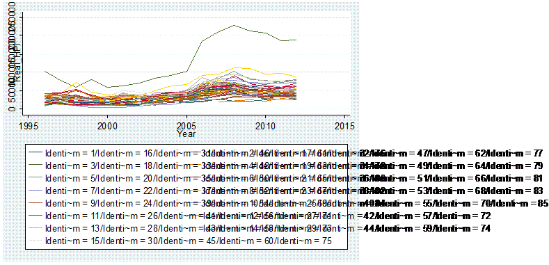 . 4. Real housing
prices of all Russian regions in 1996-2012
. 4. Real housing
prices of all Russian regions in 1996-2012
phenomenon can also be an evidence
of the fact that Russians consider real estate as real asset, which can help to
ensure the safety of capital. After the period of hyperinflation the majority
ofRussian people lost their savings and cut their consumption, however the
moment mortgage market appeared they made the great demand for such expensive
and illiquid asset as real estate. So it can be suggested that they hoped to
save the capital from another possible round of inflation. However after the
period of boom there was a period of burst - because of financial crisis in
2008-2009 real wages of Russians dropped quite dramatically, so demand for real
estate and prices plummeted as well. high volatility of prices within each
region, the difference between regions was quite high: the highest line on the graph
reflects housing prices in Moscow region and it is quite obvious that prices
there were almost 50% higher before mortgage boom in 2006 and 100% higher after
it. It is also worth mentioning that the period in study is long enough and it
covers at least two economic cycles. The sample includes two crises (in 1998
and in 2008), two period of recovery after them and one period of growth
between them. All the period can be characterized with different economic
conjuncture, different risk aversion parameters, etc. which affect both demand
and supply on real estate market.the fact that the sample is not homogenous
there is no need to get rid of outliers, because as it was mentioned before the
general population is studied.Unobservable individual characteristics can be
taken into account in the model in both cases: if there is no reason to believe
that they are correlated with independent variables and if there can be assumed
such correlation, but appropriate method of endogeniety correction is used for
coefficients assessment. statistics of all the variables are presented in the
Table 4 below.There isempirical evidence that real housing prices in Russia
were highly dispersed during the period in study - the standard deviation of
the indicator is about 56% of overall mean value.Anyway it also should be
mentioned that during the period under observation the demand for housing
(measured in square meters per person) also fluctuated significantly - for
instance in Moscow area it had rocketed up to 47% before crisis.
Table. 4.statistics of the variables
price indexes of different region
did not vary a lot, because neighbor regions usually have tight economic
connection and according to purchasing power parity prices in different regions
were more or less the same if only regional government didn’t take some
restricting actions. But there was a high intertemporal variance, because
during recessions - in 1998-2000 and in 2008-2009 there were inflation shocks
in Russia. Because of hyperinflation in some periods financial industry in
Russia could not work properly that is why loan rateduring 1996-2012 varied
from 8.4% to 147%.may wonder why the real amount of financial assets
consumption can be negative whereas the amount of current and housing
consumption is non-negative. This phenomenon goes from Russian Statistical
service methodology of financial asset value calculation. This indicator
accounts accumulated change of financial assets on year-to-year basis. During
several crises that occurred during the period of observation there were
inflation shocks when consumer prices could rose up to 200% a year so the real
value of the assets decreased because of inflation. Besides during crises
financial assets may experience significant drawdown which also diminishes
their value. As a result negative values can be observed. At the same time the
methodology of housing consumption calculation does not imply accounting for
depreciation or appreciation and therefore it can be at least zero.’s also
worth noticing that at the same time construction cost index which is
calculated as a year-on-year change of materials, machinery, details and design
costs as well as other non-salary costs of construction demonstrated very
unstable dynamics during the whole period under observation though it was
similar for all the regions (see figure5). This graph shows that time-series
data of CCI is non-stationery, which makes impossible inclusion of time-series
variation into the model because of unit root. Therefore the first difference
of this indicator should be included into the final model in order to get rid
of this problem.
Fig. 5. Construction cost index
dynamics
of the relative wage to capital
costs (CCI) also deserves attention. The graph of this indicator demonstrates
that inflation of labor cost for construction companies during past 16 years
was much more severe compared to changes in cost of materials. And it is quite
straightforward because the technology usually becomes cheaper with time - new
technologies of construction are developed, new cheaper materials are used, and
mechanization of construction becomes more widespread. At the same time labor
union pressure, development of workers’ rights protection laws, overall
increase of life quality and employees compensation after the collapse of the
Soviet Unionlead to such a rapid growth of labor cost/material cost
ratio.should be mentioned that the calculated ratio reflects only dynamic of
the labor cost/material cost indicator but not the actual value because labor
cost is approximated with real salary whereas material costs were calculated as
index. These regional time-series are also non-stationary; therefore first
differences (which have no unit roots) will be used for model estimation. The
rest of the variables are more or less stationary in time so the level of
variables will be used for estimation of theoretical model parameters
Fig. 6. Labor cost/material cost
ratio dynamics
order to identify the connection
existence between endogenous and exogenous variables the correlation
coefficients were studied. The majority of independent variables have strong
linear impact on housing prices. The signs of correlation coefficients are
mostlyin line with expected signs which comply with economic theory.
Table. 5.coefficients.
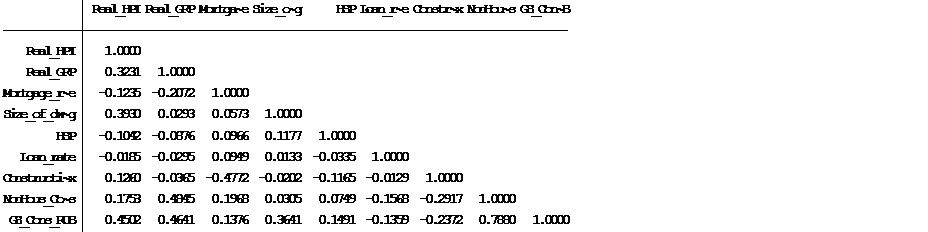
As it was assumed stricter loan
conditions negatively affect housing prices, whereasthe amount current
consumption is positively correlated to housing prices. It also can be noticed
that the state of the regional economy reflected through real GRP comparatively
strictly linked to consumption variables and to the mortgage conditions and at
the same time it is rather highly correlated with the housing prices. Despite
the fact that there is no multicollinearity in the strict sense it could be
assumed that one of these variables could be insignificant because some of them
can drag influence one from another. the components of the supply equation a
positive linear correlation between the size of dwelling and loan ratesseems to
be quite unexpected. Anyway the coefficient itself is quite small and probably
correlations can vary from region to region therefore the final conclusions
could be made only after the whole model assessment.the multicolinearity is
tested the empirical model can be estimated. The estimation of the model
parameters is implemented with help of the package of statistical analysis
Stata 12th Version. The empirical analysis of the theoretical model on the
Russian regional-level data will allow testing the significance of the whole
suggested framework of the interaction between supply and demand on the housing
market. And if the model is proved to be valid for forecasting equilibrium
states of the market, the analysis of model residuals will allow drawing some
conclusions about the possibility of non-equilibrium states. Theseresults in turn
may give a basis for further research devoted to Russian real estate market
efficiency, estimation of housing demand and supply elasticity, modeling of the
price adjustment mechanisms, etc.
estimates
model was estimated with help of
maximum likelihood method which allows to obtain consistent, asymptotically
normal and efficient (there is no alternative estimator which allows achieving
lower asymptotic variance) estimates if the sample is big enough and
Gauss-Markov conditions are fulfilled.
6. results of estimation of the
initial structural model.

Dataset was already checked for
multicolinearity, however heteroscedasticity was detected with help of
Breusch-Pagan test. The influence of heteroskedasticity can be taken into
account when assessing the significance of a particular variable by
implementing robust estimation. Anyway none of the variables changed its
significance level noticeably, so the influence of heteroscedasticity can be
considered as negligible. model as a whole is significant which means that the
joint test of all the coefficients being equal to zero allowed reject the null
hypothesis and therefore the specification of the model describes the reality
quite well. This statement can also be supported with the high R-squared of the
each equation included into the model and the overall goodness-of-fit (see
table 7 below)
.7.of-fit of the initial model.
|
Endogenous
variables
|
R^2
|
|
Ln_HP
|
39.89%
|
|
Ln_deltaH
|
11.97%
|
|
Overall
|
40.32%
|
However the results that were
obtained after model estimation appeared to be quite unexpected. First of all
due to the fact that such variable as construction cost index and wages were
taken as a first differences in order to eliminate unit root in the initial
data inclusion of trend variable (FEyear) was a bad idea, because it became
insignificant at any level. influence of regional-specific growth factor which
was approximated with help of GRP growth rate appeared to be insignificant as
well. The reason of such result may lie in the fact that there is no
significant cross-regional variation of GRP growth rate and all the regions
during the period under observation were developing along with the national
economy. And the influence of the national business cycle had already been
accounted into other variables in particular in the credit market conditions
(loan rate and mortgage rate) reflected in the variable ln_HC = .
So, both time trend and regional-specific growth rate were removed from the
initial model which allowed increasingthe goodness-of fit of the supply
equation and the whole structural model as well. most unexpected result is the
positive influence of the housing price on the households’ demand which follows
from the positive coefficient of the ln_HSP (housing stock per person)
variable. This result contradicts the basic law of demand and common sense that
higher prices restrict some households’ real estate consumption. The problem
can be caused by the wrong model specification, data features (which means that
that phenomenon really existed in Russian housing market during the period in
study) or endogeniety problem which could become a reason of biasedinconsistent
estimates and the wrong sign in the demand function. to the results of Wald
testwhich allowed testing the joint hypothesis of non equality to zero for all
the coefficients the model as a whole is significant. Therefore the first
reason of the incompliance of empirical results to economic theory can be rejected.the
same time the existence of the positive connection between the price of the
housing and the amount of housing consumption can be explained as a phenomenon
of Veblen good. That means housing can be considered as a positional good for
Russians, however this violates the main assumption of the model about rational
households’ behavior. And besides that effect usually implies the high income
of the consumers however the average real income in Russia grew with much more
moderate paces compared to the growth of housing prices. And finally there is
no statistical evidence of such phenomenon according to the linear correlation
coefficient which is negative (see Table 5) Therefore the second reason of
wrong sigh in demand function with high likelihood can be also rejected.the
existence of the endogeniety problem can be assumed. This problem can be caused
by wrong measurement of the indicator, simultaneity problem, self-selection
bias or omitted variables in the model. Due to the fact that the same indicator
was proved to be a relevant and suitable in many other research papers such as
(Kenny,1999), (Cheshire and Sheppard, 1998), (Fingleton,2008), etc. because the
results that were obtained complied totally with economic theory. So housing
stock per person can be believed as a reliable measurement of the amount of
housing available on the secondary market for a particular household. problem
means that the amount of housing changes immediately along with housing prices
fluctuations which seem to be absolutely unrealistic assumption. In average the
building process of apartment house in Russia lasts more than one year and the
assumption used in the model implies that the housing becomes available on the
secondary marketat the period which follows its commissioning. selection is a
problem which is connected to the sampling process, however due to the fact
that all the regions participate in the model estimation there actually no such
a process because general population is studied. Therefore this cause can be
rejected as well which in turn leads to the conclusion that the most possible
reason of housing quantity endigeniety is the presence of omitted variable. For
instance the availability of the land lots that are suitable for residential
construction is an important factor of housing prices and construction itself,
it can be assumed that it vary from region to region, but this indicator cannot
be directly measuredtherefore cannot be included into the model. this means
that there is a correlation between the housing stock per person and individual
error term in the model. In order to eliminate the effect sucha bias this
variable should be instrumented with help of other variables that cannot be
connected to the error term. Instrument variables have to be valid and relevant,
which means that they should be exogenous and provide high descriptive capacity
(e.g. influence significantly on endogenous variables) subject to other
Gauss-Markov’s conditions.
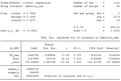
Fig. 7. FE
estimates of intermediate model
it was
assumed both regional level and national-level indicators of business cycle
appeared to be significant factors of construction activity in Russian regions
despite the fact that the absolute values of both coefficients are relatively
small.Furthermore this result also supports the statement that residential real
estate construction is a pro-cyclical variable. It is also worth noticing that
the model better describes intertemporal variation compared to cross-regional
probably because the regional-specific effect did not varied a lot across
regions but its variation precisely describes dynamics of construction in time
and at the same time an overall trend is also supposed to reflect the influence
of time effect. order to check the model for possible endogeniety consistent
fixed-effect estimators should be compared to random-effect estimators. If
there is no statistically significant difference between those two sets of
estimators then the model predicted values of housing stock per person can be
used for the estimation of the structural model. results of random effect model
estimation are presented on the figure 8 below, this model as a fixed-effect
model was checked for heteroskedasticity and as a result robust estimation was
implied. Even without testing both sets of estimators for statistical compliance
one could notice that the coefficients are almost the same which means that the
intermediate model does not cause further endogeniety and the predicted values
of endogenous variable (housing stock per person) can be used for estimation of
the structural model of Russian regional housing market.

Fig. 8. RE
estimates of the intermediate model
new variable
which was extracted out of the reduced-form model was inserted into the whole
model under the name lnHSP_hat and as it was assumed earlier this step helped
to improve the initial model significantly. The results of the new model
assessment are presented in the table 8 below.
Table 8. results of the final model
estimation

of the predicted variable allowed to
some extent eliminate the influence of endogeniety and the sign of the
coefficient before the amount of housing in the demand equation become negative
as it is required by economic theory. So at that point the model can be considered
as a suitable for further interpretation and discussion of the results.goes
without saying that the model stayed significant an all levels and what is more
the total quality of the final model improved compared to initial model for
both separate equations and the overallmodel (see table 9 below).
.9.of-fit of the final model.
|
Endogenous
variables
|
R^2
|
|
Ln_HP
|
46.02%
|
|
Ln_deltaH
|
12.31%
|
|
Overall
|
46.57%
|
Therefore it could be concluded that
the suggested theoretical framework is basically relevant however housing stock
per person which was taken as an indicator of quantity in the demand function
appeared endogenous presumably because of omitted variable. For further
research of Russian regional housing markets one should use another variable
for measurement for quantity of housing, include the indicators connected to
residential building land availability and quality of construction measurements
in the model or include an additional equation in the model which would
describe the connection of the demanded quantity of housing with other
variables that participate in the equilibration on the housing market.
of the model estimation
final model almost totally fulfilled
the expectations about all the exogenous variables influence on endogenous ones
(housing prices and net amount of residential real estate construction).
Besides, due to the fact that the model as a whole is also significant
according to rejected joint hypothesis about all coefficients being equal to
zeros it could also be concluded that the suggested paths of influence of each
of the demand-side and supply-side indicators are correctly determined as well.
model estimation approach implies that the signs of the regressions
coefficients are dictated mostly by the economic theory and less by the
researcher’s assumptions. It should be noted that all the estimated
coefficients correspond to the economic theory and most of the explored
variables appeared to be highly significant. All the components of theoretical
demand function - consumption and housing related are equally significant for
price determination. However supply function is mostly driven by housing prices
rather than cost inflation, because both components of total cost function -
labor expenses and cost of capital goods - are significant only at 5% and 10%
levels respectively.phenomenon can be explained in the following way.
Construction companies in reality are not perfectly competitive and therefore
they can have some market power to persist marginality of their business at a
stable level. Within the framework of the research companies have to reduce
construction activity and inflate prices back to the level which would keep
their operational margin stable when their total expenses increase.
The
mechanism of the interaction between housing prices and conditions on the labor
market was described in the paper of (Bover, Muellbauer, and Murphy 1989).
Authors found similar evidence of negative connection between wage level and
housing construction but the positive influence of labor cost inflation on
housing prices on the UK housing market. The wage in their model was
incorporated in both demand and in the supply functions through its inverse
relationship with unemployment level. in order to answer the question about the
power of influence of demand-side and supply-side indicators on equilibrium
housing price both direct and indirect effects should be studied. Their values
are presented in the table 10 below.
Table 10., indirect and total
effects of exogenous variables on endogenous ones

Direct effect of each variable
reflects the influence of a particular exogenous variable on corresponding
endogenous variable in the equation which contains both of them. This effect is
actually equal to the estimated coefficient in structural themodel. Indirect
effect on the other hand reflects the path of influence of exogenous variables
from one equation on the endogenous variable from another one. Total effects
are the effects that incorporate both direct and indirect ones and allow
researcher to observe the influence of all the exogenous factors on all the
endogenous ones.effect appears when the endogenous variable from one of the
equation is used for modeling the other endogenous variable. In the estimated
model housing prices that were determined within inverse demand equation
participated in the determination of net size of dwelling. Therefore the
exogenous variables from the demand function such as housing stock per person,
aggregate current consumption and the relative costs of buying real estate
coefficient indirectly affect net size of dwelling.of the most influential
housing demand factors in Russian regions is the amount of housing available on
secondary marketper one household: when this amount rises by 1 % real estate
prices drop by 0.59%. If the direct demand equationwould be constructed instead
of reverse demand function the causal relation could be inverted: when housing
prices go up by 1% the demand for residential real estate contracts by 1.69%.
fact reflects the simple idea of the law of demand and the value of the
coefficient indicates that demand for housing is price elastic. This result
supports estimation conducted by (Mayo, 1981) on state-level data for the USA
sample and partly results of the city-level research conducted by (Hanushek and
Quigley, 1980) who proved that housing demand is more elastic for relatively
expensive objects of residential real estate. is not a surprise that such
result was obtained for Russian sample because for most people housing is a
very valuable asset, often - the most valuable asset they have. So even
moderate housing price inflation which is not supported with corresponding
increase of personal income can prevent people from buying additional real
estate and make them chose other saving or consumption opportunities.conclusion
can be supported with the positive sign of the estimated coefficient of current
consumption (as it was mentioned before that it includes not only perishable
goods but some durable goods except housing as well). Anyway, taking into
account the fact that Consumption CAPM framework was used for utility function
determination and unobservable parameter delta (risk-aversion parameter) was
incorporated there it seems impossible to define the exact marginal rate of
substitution of additional living space with amount of current consumption. now
only the existence of significant positive relationship between housing prices
and amount of current consumption can be ascertained. However assessment of the
model on individual-level panel data would presumably allow estimation of the
unobserved risk-aversion parameter and drawing more precise conclusions about
the elasticity of current construction by housing prices. housing prices raise
households make their choice in favor of more current consumption - for
example, the individual may choose buying a new car over saving further in
order to buy a new flat. This can be explained with high uncertainty about the
future - there is a possibility that prices will go down - or inthe general
case that expected return on housing can be considerably less compared to
mortgage expenses, depreciation, adjustment costs, etc.costs of buying an
additional living space relative housing return are reflected in the housing
coefficient (ln_HC = ). As it was
assumed when these expenses grew and were not backed with proportionate housing
prices inflation households contracted their consumption of housing at that
period, as a result the volume demanded on real estate market dropped and
prices moderated further. Therefore it can be concluded that hypothesis H1
about negative significant influence of relative cost of buying housing on
priceswas confirmed on Russian sample. However the influence of this indicator
is much less compared to current consumption and housing stock per person: when
relative costs go up by 1% housing prices will be diminished only by 0.17%.
direct influence of time-specific and region-specific effects on housing prices
appeared insignificant due to the fact that other variables that were included
into the equation took over a quite big share of explained variance of prices.
However because of endogeniety of housing stock variable time trend and GRP
growth were used as instruments for endogenous variable and were proved to be
valid and relevant. So their influence on housing prices was accounted for
indirectly, therefore the hypothesis H2 could not be accepted unconditionally.
It should be said that housing stock is mainly prone to cyclical adjustments
and overall economic trends whereas it affects housing prices only through this
variable.the same time the most influential driver of net residential real
estate construction is housing prices themselves. The increase of prices by 1%
will encourage constructors to build 0.65% more living spaces. The positive
link between these indicators reflects the idea of the law of supply. The value
of the coefficient indicates the fact that construction is not price elastic
and it is worth mentioning that there are evidences that supply is inelastic in
some other mainly developing regions. results were obtained in papers of
(Green, Malpezzi and Mayo, 2005) who studied housing supply elasticity in large
cities of different States of the USA. Authors found the evidence that in
industrial states of the country elasticity of construction is significantly
less compared to agricultural, technological and political centers of the
country.
(Caldera and Johansson, 2013) tested
cross-country sample for presence of sustainable differences between groups of
countries that were combined according to a certain principle (geographical,
economic development level, etc.). They found that in countries with many
available residential construction land lots and weaker construction regulation
price elasticity of housing supply is relatively lower. presumable reasons of
some kind of insensitivity of construction activity to housing price dynamics
are historical (the period under observation is long enough and captures
several Soviet Union years, Perestroika years and further recovery of the
market). estate built in the Soviet Union was practically unified - within one
region and between different regions there were almost no differences in
construction style, so people had no choice but to live in standard apartments.
It is also should be mentioned that many people that days lived in the halls of
residence which were provided by government. the toughest part of the
transitional period in Russian economy privately-owned companies started
building up regions with constructions, which were distinguishable from Soviet
style of housing construction in order to cover the free market share and
fulfill appeared demand for better housing practically regardless price
situation.that time the quality of construction became higher, buildings taller
and placed with higher density in the most demanded parts of the regions due to
the fact that market became competitive. And those people who could afford
buying a new apartment created demand on primary market of real estate whereas
those who could not afford a primary real estate could buy a flat on secondary
market, which as a result pushed prices up. in turn encouraged more
construction however by the time when price instead of market share became the
matter regional market were already saturated to some extent and finding
unsatisfied demand became the bigger problem. So after the period of
construction boom prices also could be overshadowed by other factors such as
for instance availability of suitable residential construction land lots,
rising regulatory requirements and etc.other factors that were proved to be
important drivers of housing construction are construction costs. Within the
framework of the developed theoretical model they were assumed to be consisted
of labor costs which were approximated with average wage level and capital
costs which included expenses for materials, machinery, design, etc. Both of
these type of costs affect negatively construction activity which complies with
common sense and economic theory. So the hypothesis H3 can be confirmed.value
of the coefficients shows that more influential factor is capital cost
inflation because when it goes up by 1% the prices will drop by 0.35% whereas
the increase of workers’ wage by 1% will diminish housing prices by only
0.085%. Despite the fact that wage is more statistically significant and rose
more quickly compared to capital costs it should be noted that these costs
account for more than 80% of the total cost of construction. Therefore even
moderate inflation of their value can lead to considerable contraction of their
operational marginality or to increase of the prices on primary real estate
market and corresponding decrease of demand. should be noticed that as in the
case of risk-aversion parameter that was included intodemand function the
parameter alpha which reflects the marginal rate of substitution of capital
costs by labor in total costs function is also unobservable. Due to the lack of
company-level data on construction companies of each region about the structure
of their expenditures this parameter was not estimated separately of the final
coefficients of the structural model. This can be attributed to the
shortcomings of the model.variables that affect housing construction activity
indirectly (through their influence on housing prices) the most influential
factor is housing stock per person. This variable has significant negative
influence on construction activity when the indicator rises by 1% net size of
dwelling fall by 0.38%. Therefore it could be concluded that when housing
market is insufficiently saturated with living spaces construction companies
build up more actively in order to gain market share and cover potential
demand. And vise-a-versa when most areas suitable for residential construction
had been already built up companies moderate their activity or move it to other
regions where market is relatively free. influence of current consumption on
the net size of dwelling is positive and significant: when current consumption
grows by 1% construction activity increases by 0.15%. As was observed earlier
current consumption and housing prices are directly related - when housing
prices inflate households postpone housing consumption and chose other
consumption opportunities. So far it could be concluded that the higher level
of current consumption means higher housing prices,and current situation on the
market in its turn promotes formation of positive expectation by construction
companies and by this stimulates construction activity as well.of buying
residential real estate relative housing returns negatively influence net
construction. The indirect effect of this indicator is the most moderate among
all of the demand-side variables: when this ratio increases by 1% the net size
of dwelling drops by only 0.11%. And this result seems to be pretty
straightforward because this variable reflects relative cost of buying for
households not for construction companies. Due to the fact that indicator
negatively influences housing prices it acts in opposite way compared to
current consumption and facilitates the formation of negative expectations
about future prices and depresses housing construction activity. things
considered it could be concluded that all the demand-side and supply-side
factors that were included in to the theoretical model of Russian regional
housing markets some way participated in equilibrium formation process. Besides
due to the fact that the estimated structural model as a whole appeared to be
significant all the paths of influence of all indicators can be believed as
reliable and therefore used not only for further research but also for studying
the regulatory effects on the market. except discussion of direct and indirect
effects of different micro and macro indicators on housing demand and supply
one of the most interesting implication of this research is that the model
predicts equilibrium states of the system, because all the coefficients were
extracted out of interaction between prices estimated within demand function
and amount of construction dependent on these prices. The analysis of residuals
of each equation of the model will allow concluding about was the equilibrium
on housing market in Russian regions persistent at each moment of time in past
sixteen years. to the fact that the sample covers a really long period which
includes at least two whole business cycles, two severe financial crises and a
period of boom on housing market it is a question of special interest about the
rationality of economic agents that moved prices that high or that low
regarding their fundamentally justified level. It should be mentioned that by
fundamental factors hereonly those factor included into the model were meant.
the analysis of supply equation residuals were calculated as a difference
between empirical values of net size of dwelling and those estimated within the
model. The
figure 9 below represents supply equation residuals.
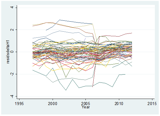
Fig.9. Residuals of supply equation.
could noticed that even though
residuals are highly dispersed for different regions which one more time
supports the idea that regions are highly heterogeneous in their economic
development they majorly do not have any trend in time and seem to be quite stable.
There are almost no significant deviations from average value for each region
and all the values lie in the close neighborhood of zero. This result tells
that the model quite precisely described variation of net construction variable
and data fits theoretical models pretty well. So it could be concluded that
supply for most regions was driven by fundamental factors even during periods
of economic instability and even the period of construction boom was consistent
with rational assumptions theory. equation residuals were calculated the same
way as supply equation residuals as a difference between empirical market data
and forecasted within the model data. The graph of their dynamics over time is
presented below.
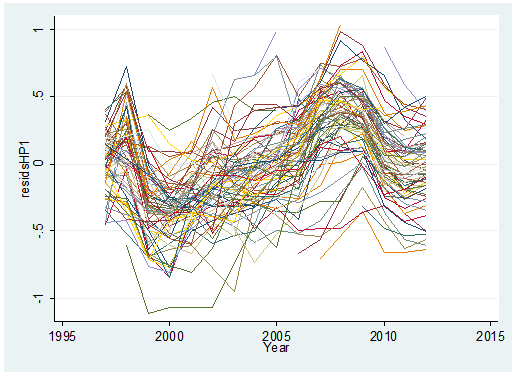
Fig.10. Residuals of supply equation
graph is much more interesting
because residuals are volatile not only over different regions but also they
are highly volatile in time. Taking into account deviations from zero there are
obvious peaks and bottoms that reflect booms and bursts on housing market in
Russia. first peak reflects the default of Russia in 1998 when there was
hyperinflation and prices rocketed up very quickly but normalized within a year
after that and even fall too much by the early 00’s. The drop in real income of
citizens and weak demand contributed to the drawdown of prices. Considering the
start of construction boom which created the situation of oversupply on the
housing market prices fall unexpectedly low and some sort of anti-bubble existed.
along with economic recovery in the country the housing market recovered
too.The following years were a period of rapid growth in many industries
including construction itself and related to it. Real income of households
increased and their savings and particularly investment in housing increased as
well. So housing market reached its equilibrium in mid-00’s but it persisted
not long because the inflation of housing prices continued up to the crisis of
2008-2009. to the model and those fundamentals on which it is based there was a
real estate bubble that time, because rapid growth of housing prices was not
supported with the corresponding rise of real disposable income, drop of
relative cost of buying additional housing or shortage of housing supply. Therefore
it can be suggested that bubble was caused by irrational behavior of households
that experienced some kind of money illusion. The link between money illusion
and housing prices was established in the paper of (Shafir, Diamond and
Tversky, 1997).market could not persist for a long time and eventually in 2008
it burst and prices experienced serious drawdown compared to their peak values.
The bubble had been over by 2010 in most regions. Several of them, presumably
regions with lowest level of income per person even experienced an anti-bubble
again. After 2010 prices stayed at their equilibrium level according to the
developed model of supply and demand on regional housing market. sum up, during
the period in observation Russian regional real estate experienced several
bubbles and even anti-bubbles which implies that price dynamics during that
time could not be explained with those factors that were included in the model.
The source of these bubbles is presumably the irrational behavior of
households. and discussion
regional housing market
All things considered quite
satisfying results were obtained - the model of equilibrium on Russian regional
housing market was constructed based on economically justified assumptions and
was proved overall significant. Therefore it could be concluded that the aim of
the study stated in the very beginning was reached. Besides, not only overall
model appeared to be relevant but each equation and both demand-side factors
and supply-side factors used for modeling equilibrium states are significant as
well.was proved on empirical data covering a long period of time that housing
prices are heavily dependent on the amount of living spaces available at the
market, other alternatives of consumption or savings and historical performance
of residential real estate as an asset class relative to the cost of buying it
such as mortgage expenses, depreciation and alternative rate of return on
financial assets.the initial indicator of housing demand - housing stock per
person - was an endogenous variable presumably connected to the availability of
spare residential land lots. It was instrumented with indicators of regional
and national business cycle, whereas these variables were excluded out of the
initial model estimation because the insignificant direct impact on housing
prices. Anyway it was proved that they participate in housing price
determination through their connection to housing construction activity.result
one more time supports the idea presented by(Leamer, 2007) that housing market
is highly connected with overall economic situation. Therefore it should be
noted that in order to avoid the problem of endogeniety the additional
indicators of residential land market need to be included into the modeling or
a different than housing stock per person indicator should be used. activity in
each region in its turn mainly orients on expected housing prices that were
assumed to be based on observed current prices. A little bit less influential
both by statistical significance and the absolute value of the regression
coefficient are cost components: labor-related and capital-related. But at the
same time the power of capital goods inflation influence is much higher
compared to wage inflation. It can be explained by the fact that expenses of the
construction companies on materials, machinery, design, etc. amount up to 80%
in overall construction costs and even moderate inflation of these costs can
have significant impact on marginality of the business. This result
particularly supports the estimates conducted by (Gyorko and Saiz, 2006) who
studied the influence of cost composition on housing supply. comparison of
fundamentally justified equilibrium housing prices forecasted within the model
and observed prices that existed on the market allowed drawing a conclusion
that housing prices periodically sharply deviated from the equilibrium state.
Peaks of these deviations match not only with crisis events such as 1998 or
2008 years when pricesdropped significantly but also considerable upward
deviation can be observed between 2005 and 2007 when there was a period of
rapid economic growth in Russia.to the fact that these leap of housing prices
was not implied by economic fundamentals it could be suggested that it was
caused by households’ irrationality and overly optimistic expectations that
lead to the housing bubble and the ensuing burst. The similar situation could
be observed on the US housing market during the pre-crisis period and according
to the conclusions of Robert Shiller presented in his book “Irrational
exuberance” (2000) one of the main reasons of that was irrational behavior of
American households. a separate important implication the relevance of the used
method of data processing can be outlined. Structural model estimation allowed
not only concluding about the factors that drive housing prices but also
determining the path through which households’ and companies’ decisions
influence equilibrium states on the using market of Russian regions. This paper
fills the gap in the research field not only because it was implemented using
structural estimation approach instead of reduced-form approach but also due to
the fact that developing Russian market was studied whereas this method of
analysis is usually used for studying developed markets (mainly the USA). are a
few limitations of this research that need to be discussed. First of all, one
of the core assumptions used for demand function modeling was that individuals
maximize their utility function which was based on consumption CAPM model. This
model can be challenged by certain number of economists that criticize the
whole concept of this model or its particular assumptions. , the strong
assumption about homogeneity of all the households was made. Within the
framework of this model all the households are rational and have same wealth
and utility function which in reality can be not that way. As in papers for
instance (Iacoviello and Neri, 2008) the individuals can be divided into
patient and impatient and their interaction on loan market might define
interest rates in the model and participate in housing equilibrium
determination process. among limitation the assumption of competitive structure
on residential real estate construction market should be mentioned. It is
implied in the model that construction companies have the same total cost
function and they are price-takers on both housing and resources markets. This
condition was used for simplification of the calculations, but in reality the
industry structure can be different in each region. The construction companies
also may compete not only within one region but also on cross-regional market
and this kind of interaction was also omitted.it should be noticed that the
lack of individual-level and company-level data did not allowed the estimation of
such unobservable variables as risk-aversion parameter (denoted in the model as
delta) and marginal rate of substitution of capital by labor (denoted in the
model as alpha). These parameters in the estimated model were incorporated into
assessed coefficients of corresponding variables.following suggestions for
further research in the field can be outlined. First of all a straightforward
approach of endogeniety elimination can be suggested - simply to include some
variables that were considered as omitted in this research. Among them could be
the amount of spare land appropriate for residential construction, an average
price of square meter of this land, probably other qualitative characteristics
of constriction in particular connected to air quality, neighborhood, etc. Also
the influence of strictness of construction regulation and some measures of
bureaucratic difficulties can be taken into account. , as was mentioned earlier
instead of competitive structure of construction industry other forms of competition
can be modeled and more realistic and comprehensive picture of housing price
driver can be obtained. to the fact that according of the model estimators
there were a serious deviations of housing prices from equilibrium the whole
separate research can be devotedto understanding this phenomenon. Besides, one
also could try to measure theconvergence speed towards equilibrium with help of
error correction model.
list of references
Aoki,
Kosuke, James Proudman, and Gertjan Vlieghe. 2004. “House Prices, Consumption,
and Monetary Policy: A Financial Accelerator Approach.” Journal of Financial
Intermediation 13 (4): 414-35. , Patrick, Phoebe Chan, Dirk Krueger, and Daniel
Miller. 2013. “A dynamic model of housing demand: estimation and policy
implicatios” International Economic Review 54 (2): 409-442., Michael. 1973.
“Recent Empirical Work on the Determinants of Relative House Prices.” Urban
Studies 10 (2): 213-33.J. J. et al. Optimal Durable and Nondurable Consumption
with Transactions Costs. - Board of Governors of the Federal Reserve System
(US), 1993. - №. 93-12., Olympia, John Muellbauer, and Anthony Murphy. 1989.
“Housing, Wages and UK Labour Markets.” Oxford Bulletin of Economics and
Statistics 51 (2): 97-136.
Caldera,
Aida, and Åsa Johansson. 2013. “The Price Responsiveness of Housing
Supply in OECD Countries.” Journal of Housing Economics 22 (3): 231-49.
Calomiris,
Charles W., Stanley D. Longhofer, and William R. Miles. 2013. “The
Foreclosure-House Price Nexus: A Panel VAR Model for U.S. States, 1981-2009:
The Foreclosure-House Price Nexus.” Real Estate Economics 41 (4).D., Helsley
R., The fundamentals of land prices and urban growth, Journal of Urban
Economics, Volume 26, Issue 3, 1989, Pages 295-306. , Karl E., and Robert J.
Shiller. 1988. The Efficiency of the Market for Single-Family Homes. National
Bureau of Economic Research Cambridge, Mass., USA., Pietro, Nathalie Girouard,
Christophe André, and Robert Price. 2004. “Housing Markets, Wealth and
the Business Cycle.” OECD Economics Department Working Papers 394.
Cheshire
P., Sheppard S. Estimating the demand for housing, land, and neighbourhood
characteristics //Oxford Bulletin of Economics and Statistics. - 1998. - Т.
60. - №. 3. - С. 357-382.B. A.,
Heathcote C. R., O'Neill T. J. Estimating cohort health expectancies from cross‐sectional
surveys of disability //Statistics in Medicine. - 2001. - Т.
20. - №. 7. - С.
1097-1111.DiPasquale, William C. Wheaton, Housing Market Dynamics and the
Future of Housing Prices, Journal of Urban Economics, Volume 35, Issue 1, 1994,
Pages 1-27, Marjorie. 2001. “Owner-Occupied Housing in the Presence of
Adjustment Costs: Implications for Asset Pricing and Nondurable Consumption.”
Manuscript, UCSD.B. Housing supply, housing demand, and affordability //Urban
Studies. - 2008. - Т.
45. - №. 8. - С. 1545-1563.,
Andreas, and Basit Zafar. 2014. “The Sensitivity of Housing Demand to Financing
Conditions: Evidence from a Survey.” FRB of New York Staff Report, no. 702, Li,
and Qinghua Zhang. 2013. “Market Thickness and the Impact of Unemployment on
Housing Market Outcomes.” National Bureau of Economic Research., Andra C., and
Michael T. Owyang. 2010. “Is Housing the Business Cycle? Evidence from US
Cities.” Journal of Urban Economics 67 (3): 336-51., Edward L., Joseph Gyourko,
and Albert Saiz. 2008. “Housing Supply and Housing Bubbles.” Journal of Urban
Economics 64 (2): 198-217., Allen C. 1978. “Hedonic Prices, Price Indices and
Housing Markets.” Journal of Urban Economics 5 (4): 471-84.R. K., Malpezzi S.,
Mayo S. K. Metropolitan-specific estimates of the price elasticity of supply of
housing, and their sources //The American Economic Review. - 2005. - Т.
95. - №. 2. - С. 334-339., Arthur,
and Andrew Aitken. 2010. “Housing Supply, Land Costs and Price Adjustment.”
Real Estate Economics 38 (2): 325-353.J., Saiz A. Construction costs and the
supply of housing structure* //Journal of regional Science. - 2006. - Т.
46. - №. 4. - С. 661-680.E. A.,
Quigley J. M. What is the price elasticity of housing demand? //The Review of
Economics and Statistics. - 1980. - С.
449-454., Hideaki, M. Ayhan Kose, Christopher Otrok, and Marco E. Terrones.
2012. “Global House Price Fluctuations: Synchronization and Determinants.”
National Bureau of Economic Research.S., Jones N. House prices since the 1940s:
cointegration, demography and asymmetries //Economic Modelling. - 1997. - Т.
14. - №. 4. - С. 549-565., Min,
and John M. Quigley. 2006. “Economic Fundamentals in Local Housing Markets:
Evidence from US Metropolitan Regions.” Journal of Regional Science 46 (3):
425-453., Matteo. 2004. “Consumption, House Prices, and Collateral Constraints:
A Structural Econometric Analysis.” Journal of Housing Economics 13 (4).,
Matteo. 2005. “House Prices, Borrowing Constraints, and Monetary Policy in the
Business Cycle.” American Economic Review, 739-764., Matteo. 2010. Housing in
DSGE Models: Findings and New Directions. Springer, Matteo M., and Stefano
Neri. 2008. “Housing Market Spillovers: Evidence from an Estimated DSGE Model.”
National Bank of Belgium Working Paper, no. 145., Deniz, and Prakash Loungani.
2012. “Global Housing Cycles.”, Keith, and Tom Mayock. 2014. “Housing Bubbles
and Busts: The Role of Supply Elasticity.” Land Economics 90 (1): 79-99.A.
Expected returns on major asset classes. - 2012.G. Modelling the demand and
supply sides of the housing market: evidence from Ireland //Economic Modelling.
- 1999. - Т. 16. - №. 3. - С.
389-409., N. Kundan, and Hardik A. Marfatia. 2016. “The Dynamic Relationship
Between Housing Prices and the Macroeconomy: Evidence from OECD Countries.” The
Journal of Real Estate Finance and Economics, January., John, and James A.
Wilcox. 2013. “Evidence and Implications of Regime Shifts: Time-Varying Effects
of the United States and Japanese Economies on House Prices in Hawaii: Regime Shifts
in Real Estate Markets.” Real Estate Economics 41 (3)., Edward E. 2007.
“Housing Is the Business Cycle.” National Bureau of Economic Research.,
Stephen, and others. 2003. “Hedonic Pricing Models: A Selective and Applied
Review.” Section in Housing Economics and Public Policy: Essays in Honor of
Duncan Maclennan.N. G., Shapiro M. D. Risk and return: Consumption versus
market beta. - 1984.S. K. Theory and estimation in the economics of housing
demand //Journal of Urban Economics. - 1981. - Т.
10. - №. 1. - С. 95-116.A., Supply
constraints and housing market dynamics, Journal of Urban Economics, Volume 77,
September 2013, Pages 11-26N., Westaway P. Modelling structural change in the
UK housing market: a comparison of alternative house price models //Economic
Modelling. - 1997. - Т.
14. - №. 4. - С. 587-610., James
M. 1984. “Tax Subsidies to Owner-Occupied Housing: An Asset-Market Approach.”
The Quarterly Journal of Economics 99 (4): 729.J. M., Weil D. N., Shiller R.
House price dynamics: the role of tax policy and demography //Brookings Papers
on Economic Activity. - 1991. - Т.
1991. - №. 2. - С.
143-203., Sherwin, and Robert H. Topel. 1986. A Time-Series Model of Housing
Investment in the US. National Bureau of Economic Research Cambridge, Mass.,
USA.E., Diamond P., Tversky A. Money illusion //The Quarterly Journal of
Economics. - 1997. - С.
341-374.R. J. Irrational exuberance //Princeton UP. - 2000., Kostas, and Haibin
Zhu. 2004. “What Drives Housing Price Dynamics: Cross-Country Evidence.” BIS
Quarterly Review, March., Mr Jerome, Ms Ursula Vogel, and Ms Enrica
Detragiache. 2012. Macroprudential Policies and Housing Prices A New Database
and Empirical Evidence for Central, Eastern, and Southeastern Europe. 12-303.
International Monetary Fund. , Wolf. 2008. “The Homogenization of the Financial
System and Financial Crises.” Journal of Financial Intermediation 17 (3),
Nafeesa, and Peggy E. Swanson. 2013. “A Closer Look at the U.S. Housing Market:
Modeling Relationships among Regions: A Closer Look at the U.S. Housing
Market.” Real Estate Economics 41 (3)
Appendix
of research papers based on
reduced-form models
|
Article
attributes
|
Sample
|
Variables
|
Results
|
(Hirata
et al. 2012)
“Global
House Price Fluctuations: Synchronization and Determinants”
IMF
Working paperSample:
18 advanced OECD (Organization for Economic Cooperation and) countries;period:
quarterly series from January 1971 to March 2011Housing prices determinants:
GDP, equity prices, credit, short- and long-term interest rates
|
Method: Factor Augmented Vector Autoregression
(FAVAR)Authors found the evidence of strong linear relationship between
housing prices and credit conditions, but no evidence of intertemporal
interaction between housing prices and business cycle, equity market movements
and interest rates.
|
|
|
|
(Igan
and Loungani 2012)
“Global
Housing Cycles” Working paper Sample: 22 advanced countries;period: different
for each country (quarterly data)Housing prices determinants: lagged
affordability; Income per capita growth rate; working-age population growth
rate; equity market growth rate; credit growth rate; short-term interest rate;
long-term interest rate
|
Method:
Pooled OLS regressionHousing
affordability negatively affects real estate return for more than eighty
percent of observed regions. Besides change in personal disposable income was
proved as a significant factor of pushing prices up. There is also a positive
relation between house price changes and population growth.
|
|
|
|
(Vandenbussche,
Vogel, and Detragiache 2012)
“Macroprudential
Policies and Housing Prices-A New Database and Empirical Evidence for Central,
Eastern, and South-Eastern Europe”
IMF
Working paperSample:
16 CESEE countries (including Russia);period: different for each country but
generally beginning from 2000 (quarterly data).Housing prices determinants: GDP
per capita, Domestic real interest rate; Foreign real effective interest rate;
Working population data; Macroprudential policy measures (for Russia only
liquidity measures such as reserve requirements rate on fc and lc deposits and
reserve requirements base): Fixed-effect OLS regressionRussia has an almost
flat curve of macroprudential policy indicator constructed by authors, so this
factor was not proved to be important, however for majority of other countries
the changes of macropolicy led to shocks on housing markets.
|
It was proved that after shock prices are tend
to converge towards equilibrium rather fast. Moreover there was determined an
intertemporal dependency structure of housing prices. Estimates for lagged
changes in per capita GDP and interest rates, changes in working-age
population are not significant
|
|
|
|
(Calomiris,
Longhofer, and Miles 2013)
“The
foreclosure-house price nexus: a panel VAR model for U.S. states, 1981-2009”
Real Estate Economics. - 2013. - Т. 41. - №.
4. - С.
709-746.Sample: all the states of the USA
Time
period: 1989-2009 (quarterly data)Housing prices determinants:
growth of home prices, foreclosure rate; growth rates of employment,
single-family permits, existing home sales,
|
Method: Panel Vector Autoregression
(PVAR)Foreclosure and housing prices are highly correlated with each other. This
dependence results from the fact that housing is collateral for the mortgage
and housing price shocks disturb credit market and these conditions in turn
affect prices. Foreclosures negatively impact home prices. But the negative
impact of prices on foreclosures is larger. The variance decompositions show
that prices explain 16% of the variation in, while foreclosures explain only
5% of the variation in prices.
|
|
|
|
(Krainer
and Wilcox 2013)
“Evidence
and Implications of Regime Shifts: Time‐Varying
Effects of the United States and Japanese Economies on House Prices in Hawaii”
Real Estate Economics. - 2013. - Т. 41. - №.
3. - С.
449-480.Sample: Real House Price Indexes in Hawaii, in the USA and in Japan
Time
period: 1976-2008 (annual data)Housing prices determinants: demand
factors such as relative housing prices (US/ Hawaii and Japan/Hawaii), Stock
prices, Net Worth, GDP, Net Worth*High income share
|
Method: Constant-coefficient model VS
Time-Varying coefficient modelThe time-varying coefficient model appeared to
be significantly better than constant-coefficient model, so the regime shift
existed. Relative house prices, Net Worth, GDP and Net Worth*High income
share appeared to be significant for housing price index determination.
|
|
|
|
(Fuster
and Zafar 2014)
“The
Sensitivity of Housing Demand to Financing Conditions: Evidence from a Survey”
FRB of New York Staff Report. - 2014. - №. 702.Sample: 1211 household heads in
the USA
Time
period: 2014 (monthly data)Housing prices determinants: change
of down payment, non-housing wealth shock and change of mortgage rate
Method:
OLS (panel regression)of mortgage conditions (such as
decrease of down payment) and external increase of income positively influence
constructed by authors indicator “willingness to pay” (WTP). This effect is
higher for households with income lower than the median in the sample. However the
influence of particularly mortgage rate is moderate.