־G).
Therefore: S=I+NX or S-I=NX where S-I denote net capital outflow and NX is
trade balance of a country. In case when S>I is increase in foreign
purchases of home assets which means claim on future output of home
country.formulate a model for a small open economy I use four assumptions:,
production of goods and services in the small open economy consists of three
sectors, consumption goods. investment goods, and government services.,
production function of each of the sectors includes capital and labor in
different proportions in linear homogeneous production functions (Hodrick,
1980):
=F(K,L)
, investment (I) is inversely
related to the interest rate: I=I(r), consumption is positively lined with
disposable income:
=C(Y-T)
yields:
NX=(Y-C-G)-I; NX = S-I; NX =
Y-C(Y-T)-G-I(r*)
where
r* denotes world interest rate. As Italy is a small open economy with perfect
capital mobility the interest rate in Italy (r) is equal to the world interest
rate (r*) (Figure 2).
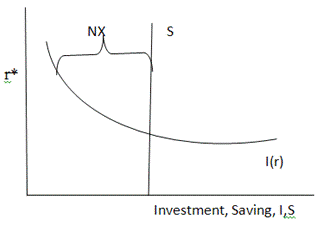 2 - Saving and
Investment in Italy, small open economy
to Barnett and Brooks (2010) when
government implement fiscal policy at home or increases G it leads to decrease
in national savings, as Italy takes world interest rate as given investment
stays at the same level unchanged. Using macroeconomic data for Italy I can
test the validity of fiscal policy at home on Italy. As it can be seen in the
scatterplot there is negative relationship between G and S (Figure 3). The
Italian macroeconomic data perfectly fits theory of fiscal policy at home in a
small open economy. Implementation of fiscal policy that causes reduction in
savings (S) shifts saving curve and leads to trade deficit (Figure 4). This is
confirmed by existing macroeconomic data for Italy during 2001 - 2010 (Figure
5). As savings in Italy decreased from 40 billion dollars to below zero during
2001 - 2010 net export (NX) has followed the same pattern.another case when
fiscal policy takes place outside of Italy and other countries increase their
government expenditures. It leads to reduction in global saving level and
interest rate increases. Thus it further initiates reduction in investment and
creates trade surplus (Figure 6).
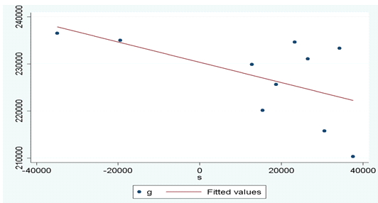 3 - Government
expenditure (G) and saving (S) scatterplot
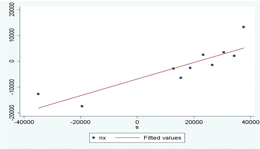 4 - Net export (NX)
and saving (S) scatterplot
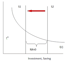 5 - Fiscal
expansion in Italy
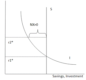
Figure 6 - Fiscal expansion outside
of Italy
1.2 USA
line with finding of Cooper (1985)
the economy of the USA is a large open economy. It constitutes 23% of global
production and is more than 2 times greater than the second largest economy
(Japan) (Figure 7). Another argument in favor fact that the USA is a large open
economy is a number of studies that found that inflation rates in the USA are
important determinants of inflation volatility in other countries (Cheung and
Yuen, 2001). However Mankiw (2009) argues that macroeconomic analysis of the
USA must be carried out implementing a mix of closed economy and small open
economy.presence of assumption of closed economy the loanable market
equilibrium in the USA can be expressed as (Figure 6b). Equilibrium interest
rate is determined when the S=I in the loanable market. In case of increase in
savings the S curve shifts to the left causing increase in interest rate. As
interest rate in the economy of the USA determines the investment level, former
starts to decrease.
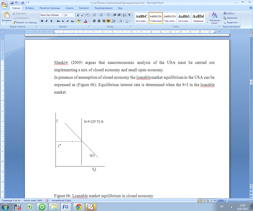 7 - Loanable market
equilibrium in closed economy
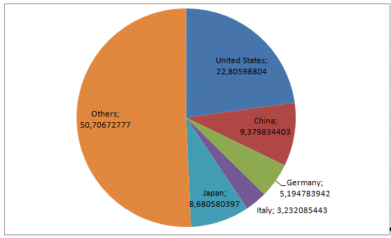 8 - Major global
economies by their respective shares, 2011
2. Short run models
Long run economic models do not
reveal that GDP and GDP per capita grow cyclically. Economic growth in Italy
and the USA has not been stable during 2001 - 2010. Both countries experienced
significant economic slowdowns in 2007-2009 when the GDP growth rate fell
significantly below zero (Figure 8). In economic studies such fluctuations in
economic growth and other macroeconomic indicators are called business cycles
(Mankiw, 2009). Among the most successful business cycle models are Okun’s Law
and Philips curve. Many studies have successfully recovered the results in
cross country studies and Okun’s Law became part of macroeconomic textbook
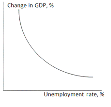
models (Ball et al, 2012). The inverse relationship between economic growth and
unemployment level is determined by Okun’s Law (Figure 9).
2.1 Italy
this section I will estimate Okun’s
Law for the Italian economy. A number of other studies have focused on
estimation of this economic relationship within Europe and for selected
countries (Stock, 2010). McKinsey (2011) doesn’t recover the Okun’s Law in his
cross country econometric studies. The author concludes that relationship
doesn’t hold due to labor market mismatches. The Okun’s Law can be expressed
as:
=a1+a2*RGDP_Gi+ei,
unemp - is change in unemployment
rate, RGDP_G is real GDP growth, e - error term.visual representation of the
Okun’s Law shows that overall the economic relationship between unemployment
and GDP growth holds in Italy during 2001 - 2010. It should be noted that
during that period an outlier has been detected when unemployment rate was 7.8%
and economic growth was significantly below zero. This is explained by the
recession in the global economy in 2008 (Figure 10, right panel).
2.2 USA
’s Law has been successfully used in
a number of economic studies devoted to the unemployment problem in the USA
(Owyang and Sekhposyan (2012). Owyang and Sekhposyan (2012) estimate Okun’s Law
for the USA using quarterly data covering 1947 - 2011 and incorporate a number
of recession dummies. The authors recover the results of Okun (1962) and
Plosser and Schwert (1979). I follow the estimation of Okun (1962) and estimate
the Okun’s Law for the USA using annual data for 1980 - 2010. As it can be seen
there is strong negative link between the unemployment change and output growth
in the USA (Figure 10, left panel).estimation through implementing OLS method
shows that the statistical relationship between change in unemployment and GDP
growth is:in unemployment = 7.07-0.26*GDP_Growthmodel of aggregate demand that
explains output changes in the short run is the IS-LM model (Mankiw, 2009). The
IS-LM model consists of two parts: IS - representing goods market and LM -
money market. Following previous section on long run models I derive planned
expenditure as:
=C+I+G (1)=C(Y-T) (2)=I* (3)=G*
(4)=T* (5)
Combining (2), (3), (4) and (5) in
(1) gives:
=C(Y-T*)+I*+G* (6)
equilibrium is achieved when PE=Y or
planned expenditure matches actual (Figure 11).in the economy is a function of
interest rate (Dupor, 2001): I=I(r) (7).the IS curve for Italian and US economy
can be graphically derived based on equations (6) and (7) (Figure 12).
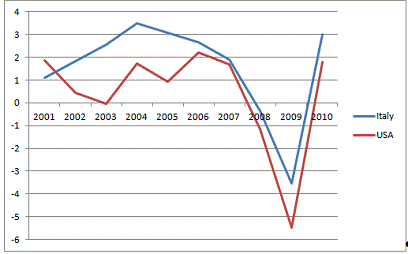 9 - GDP growth rate
in Italy and the USA, 2001- 2010
 10 - Okun’s Law
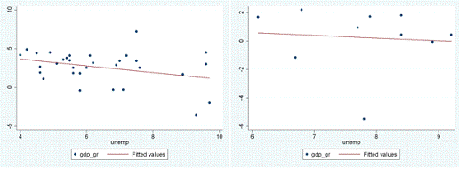
Figure 11 - Okun’s Law in the USA
(left panel) and Italy (right panel), selected year
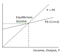 12 - Keynesian
Cross
economy italy model
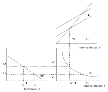 13 - Derivation of
IS Curve for Italy and the USA
Derived model can has been used to
see how economy reacts to changes in fiscal policy. Assume Italian government
increases its government expenditure (G) by 4 billion dollars, as it happened
in 2000. Increase in G shifts up PE curve up and leads to rightward shift of
the IS curve at a given interest rate and causes increase in output. Based on
the macroeconomic statistics of the Italy it can be seen that in the highest
increase in G has occurred in 2000, which followed by the largest economic
expansion since 1991 (Table 2). The existing statistical evidence supports the
framework of ISLM model for developed countries such as Italy and the USA.
2 - Annual growth in GDP and
Government Expenditure in Italy
|
1991
|
1992
|
1993
|
1994
|
1995
|
1996
|
1997
|
1998
|
1999
|
2000
|
|
G, growth (%)
|
1.9
|
0.95
|
-1.7
|
-3.2
|
0.8
|
0.5
|
0.4
|
1.4
|
2.2
|
|
Y, growth (%)
|
1.5
|
0.8
|
-0.9
|
2.2
|
2.8
|
1.1
|
1.9
|
1.5
|
1.5
|
3.7
|
framework of LM emerges directly
from the theory of liquidy preference. According to the theory the level of
real money balances supply is fixed:
/P=M*/P* (8)
level of money supply is determined
by the central bank of the USA. The level of P is fixed as we assume sticky
prices in the short run (Guesnerei, 2001). On the other hand demand for the
money is:
(M/P)d =L(r) (9)
the Italian equlibrium interest rate
is given when (8) = (9) or demand for money ballances matches supply (Figure
13).
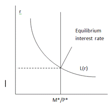 14 - The theory of
liquidity preference
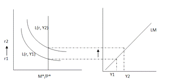 15 - Derivation of
LM curve
on the derivation of the LM curve it
can be concluded that reduction in the money supply for existing level of
output shifts the LM curve and increases equilibrium interest rate of the money
market. This is confirmed by King and Watson (1995).illustrate the impact of
reduction in money supply in interest rate on Italy and USA I will use Money
and quasi money growth (annual %) as a proxy for money supply and real interest
rate as a proxy for interest rate. The scatterplot below illustrates the
relationship between the money supply reduction and interest rate in the
framework of ISLM model during 2000 - 2010 for Italy and the USA (Figure 15).
As it can be seen the relationship doesn’t hold for the specified period.
Overall the money supply has been increasing along with the real interest rate.
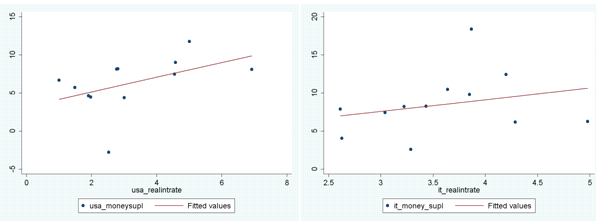
Figure 16 - LM relationship for USA
and Italy during 2000 -2010
if the data is extended to 1961 -
2009 the relationship exists in the long run (Figure 16). Reduction in the
money supply Italy has increased interest rate (left panel in Figure 16). The
results are in line with the assumptions of the IS LM model.
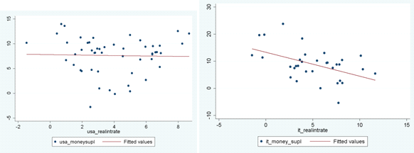
Figure 17 - LM relationship for USA
and Italy during 1961-2010
that in 2011 the European Central
Bank started to sell its foreign currency reserves and buy Euros. How would
this affect economies of Portugal and China? Use models above to illustrate you
answer.Central Banks makes a decision to support European currency the ECB
engages in purchasing Euros on the FX market. It reduces money supply. The
reduction in money supply leads to increase in interest rate. Supply of Euros
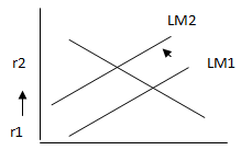
on the foreign market decreases and Euro becomes strong on the FX.case of
Italy, LM shits right and IS remains the same leading to increase in interest rate
(figure 17). As the interest rate increases investment fall as I=I(r). Decrease
in money supply leads to upward pressure on the interest rate, capital inflows
in the Italy as inverstors are seeking higher returns. Capital inflow controls
increase in interest rate to the ceiling or r*. Investing in Italy requires
conversion of the foreign currency into Euro hence appreciating it further. As
the Euro becomes stronger the Export decline due to inverse relationship
between exchange rate and net exports: NX = NX(e). Output in Italy declines and
makes Italian goods more expensive on the global market.
 18 - Decrease in
domestic money supply.
case of China the exchange rate of
the Chinese currency will depreciate (Figure 18) and become weaker compared to
Euro. Thus increase in the money supply of foreign currency stimulates export
of Chinese goods as they become cheaper compared to the Italian. Increase in
net exports will stimulate increase in income in the Chinese economy.
Conclusion
this I have estimated a long run and
short run models for the economies of the USA and Italy. For the choice of long
run models I have used small open economy and small closed economy. The
statistical evidence from the macrodata for these countries is in line with the
theory. Fiscal policy at home leads to increase in G and decrease in S and
trade deficit during 2001- 2010 whereas fiscal policy abroad leads to increase
in interest rate.case of short run model. First I have tested Okun’s Law which
can be expressed as inverse relationship between economic growth and
unemployment change. The existing macroeconomic data for Italy and the USA once
again support existence of this economic link in the countries. As a final step
I derived ISLM model for both economies. Based on the macroeconomic statistics
of the Italy it can be seen that in the highest increase in G has occurred in
2000, which followed by the largest economic expansion since 1991 (Table 2).
The existing statistical evidence supports the framework of ISLM model for
developed countries such as Italy and the USA.
References
1. Mankiw
N. Gregory. 2009. Macroeconomics. Seventh Edition. Worth Publishers.
2. Hodrick,
Robert J. "Dynamic effects of government policies in an open
economy." Journal of Monetary Economics 6.2 (1980): 213-239.
. Cooper,
Richard N. The United States as an open economy. Harvard Institute of Economic
Research, 1985.
. Cheung,
Yin-Wong, and Jude Yuen. "Effects of US inflation on Hong Kong and
Singapore." Journal of Comparative Economics 30.3 (2002): 603-619.
. Ball,
Laurence M., Daniel Leigh, and Prakash Loungani. Okun's Law: Fit at Fifty. No.
w18668. National Bureau of Economic Research, 2013.
. Stock,
Luisa, and Kurt Vogler-Ludwig. "NAIRU and Okun’s Law-The Macro-Economy in
a Nutshell? Final report." (2010).
. McKinsey
Global Institute (2011), “An Economy That Works: Job Creation and America’s
Future”, June 2011 report
. Owyang,
Michael T., and Tatevik Sekhposyan. "Okun’s law over the business cycle:
was the great recession all that different?." Federal Reserve Bank of St.
Louis Review 94.5 (2012): 399-418.
. Dupor,
Bill. "Investment and interest rate policy." Journal of Economic
Theory98.1 (2001): 85-113.
. Guesnerie,
Roger. "Short-run expectational coordination: Fixed versus flexible
wages." The Quarterly Journal of Economics 116.3 (2001): 1115-1147.
. King,
Robert G., and Mark W. Watson. "Money, prices, interest rates and the
business cycle." The Review of Economics and statistics (1996): 35-53.
12. Shamsadìni,
Solmaz, Reza Moghaddasì. "Relationship Between Trade Openness and
GDP Growth a Panel Data Analysis." World
Applied Sciences Journal 8.7 (2010): 906-911.
. Barnett,
Steven Alan, and Ray Brooks. China: does government health and education
spending boost consumption. No. 2010-2016. International Monetary Fund, 2010.